Cleaning Summary: Treasury Bond Returns#
import sys
from pathlib import Path

sys.path.insert(0, "../../src")
sys.path.insert(0, "./src")

import calc_treasury_bond_returns
import pandas as pd

# import polars as pl
from he_kelly_manela import pull_he_kelly_manela
from settings import config

DATA_DIR = Path(config("DATA_DIR"))
Treasury Bond Returns Summary#
By leveraging the TRACE dataset from openbondassetpricing.com, the FTSFR dataset ensures a robust foundation for analyzing treasury bond returns, adhering to established methodologies and incorporating comprehensive data cleaning procedures.
Data Cleaning and Construction#
The treasury bond returns dataset is constructed using the following cleaning and processing steps:
1. Bond Selection Criteria#
CUSIP Filtering:
Only include bonds with CUSIPs starting with ‘91’ (indicating Treasury securities)
This ensures we’re only analyzing genuine Treasury bonds
2. Return Processing#
Return Conversion:
Convert raw returns to decimal form by dividing by 100
This standardizes the return format for analysis
Return Filtering:
Remove observations where returns exceed 50% (tr_return > 0.5)
This eliminates potential data errors or extreme outliers
3. Maturity Grouping#
Maturity Bins:
Create 10 maturity groups using 0.5-year intervals from 0 to 5 years
Bins: [0.0, 0.5, 1.0, …, 5.0]
Each group represents a specific maturity range for analysis
Group Assignment:
Assign each bond to a maturity group based on its time to maturity (tau)
Drop observations with missing maturity information
Convert group labels to integers for easier analysis
4. Portfolio Construction#
Return Aggregation:
Group bonds by date and maturity group
Calculate mean returns for each group
This creates a time series of portfolio returns for each maturity group
5. Data Quality Checks#
Missing Value Handling:
Remove observations with missing returns
Remove observations with missing maturity group assignments
Outlier Treatment:
Extreme returns (>50%) are filtered out
This ensures the analysis focuses on normal market conditions
This cleaning process ensures a high-quality dataset for analyzing Treasury bond returns across different maturity groups, facilitating comparison with the Kelly-Manzello data.
hkm = pull_he_kelly_manela.load_he_kelly_manela_all(
    data_dir=DATA_DIR / "he_kelly_manela"
)
treas_hkm = hkm.iloc[:, 34:44].copy()
treas_hkm["yyyymm"] = hkm["yyyymm"]
treas_hkm.head()
treas_hkm.tail()
treas_hkm.describe()
treas_hkm.isnull().sum()
US_bonds_01    25
US_bonds_02    25
US_bonds_03    25
US_bonds_04    25
US_bonds_05    25
US_bonds_06    25
US_bonds_07    25
US_bonds_08    25
US_bonds_09    25
US_bonds_10    25
yyyymm          0
dtype: int64
treas_bond_returns = calc_treasury_bond_returns.calc_returns(
    data_dir=DATA_DIR / "us_treasury_returns"
)
treas_bond_returns.describe()
| DATE | 1 | 2 | 3 | 4 | 5 | 6 | 7 | 8 | 9 | 10 | |
|---|---|---|---|---|---|---|---|---|---|---|---|
| count | 668 | 668.000000 | 668.000000 | 668.000000 | 665.000000 | 665.000000 | 665.000000 | 668.000000 | 668.000000 | 665.000000 | 659.000000 |
| mean | 1997-11-14 12:25:52.095808384 | 0.003809 | 0.004242 | 0.004447 | 0.004466 | 0.004474 | 0.004838 | 0.005006 | 0.005152 | 0.005141 | 0.005120 |
| min | 1970-01-31 00:00:00 | -0.000283 | -0.008939 | -0.025195 | -0.032362 | -0.046647 | -0.052993 | -0.052765 | -0.060457 | -0.058666 | -0.059056 |
| 25% | 1983-12-23 06:00:00 | 0.001228 | 0.000874 | 0.000446 | 0.000224 | -0.000375 | -0.000747 | -0.001473 | -0.002057 | -0.002714 | -0.003201 |
| 50% | 1997-11-15 00:00:00 | 0.003798 | 0.003604 | 0.003525 | 0.003321 | 0.003453 | 0.003900 | 0.004090 | 0.004340 | 0.004370 | 0.004511 |
| 75% | 2011-10-07 18:00:00 | 0.005326 | 0.006152 | 0.007166 | 0.007829 | 0.008772 | 0.010052 | 0.011202 | 0.012094 | 0.012924 | 0.013117 |
| max | 2025-08-31 00:00:00 | 0.023142 | 0.045551 | 0.064735 | 0.068330 | 0.091789 | 0.095415 | 0.086319 | 0.093149 | 0.093774 | 0.121050 |
| std | NaN | 0.003098 | 0.004619 | 0.006256 | 0.007471 | 0.008891 | 0.010458 | 0.011638 | 0.012975 | 0.013851 | 0.014982 |
Comparing FTSFR with He Kelly Manela#
# Print initial data info
print("Treasury Bond Returns Info:")
print(treas_bond_returns.info())
print("\nTreasury Bond Returns Head:")
print(treas_bond_returns.head())
print("\nTreasury Bond Returns Date Range:")
print(treas_bond_returns["DATE"].min(), "to", treas_bond_returns["DATE"].max())

print("\nHKM Treasury Bonds Info:")
print(treas_hkm.info())
print("\nHKM Treasury Bonds Head:")
print(treas_hkm.head())

# Convert treas_hkm dates to datetime
treas_hkm["date"] = pd.to_datetime(
    treas_hkm["yyyymm"].astype(int).astype(str), format="%Y%m"
) + pd.offsets.MonthEnd(0)

print("\nAfter date conversion - HKM Treasury Bonds Head:")
print(treas_hkm.head())
print("\nHKM Treasury Bonds Date Range:")
print(treas_hkm["date"].min(), "to", treas_hkm["date"].max())

# Convert treas_bond_returns DATE to datetime if it's not already
treas_bond_returns["DATE"] = pd.to_datetime(treas_bond_returns["DATE"])

print("\nAfter date conversion - Treasury Bond Returns Head:")
print(treas_bond_returns.head())
print("\nTreasury Bond Returns Date Range:")
print(treas_bond_returns["DATE"].min(), "to", treas_bond_returns["DATE"].max())

# Try the merge
merged_df = pd.merge(
    treas_bond_returns, treas_hkm, left_on="DATE", right_on="date", how="inner"
)

print("\nMerged DataFrame Shape:", merged_df.shape)
print("\nMerged DataFrame Head:")
print(merged_df.head())

# Create subplots for each pair of columns
import matplotlib.pyplot as plt

if not merged_df.empty:
    fig, axes = plt.subplots(5, 2, figsize=(15, 20))
    axes = axes.flatten()

    for i in range(10):
        col1 = str(i + 1)  # Column from treas_bond_returns
        if i == 9:
            col2 = "US_bonds_10"  # Column from treas_hkm
        else:
            col2 = f"US_bonds_0{i + 1}"  # Column from treas_hkm

        ax = axes[i]
        ax.plot(
            merged_df["DATE"], merged_df[col1], label=f"Portfolio {i + 1}", color="blue"
        )
        ax.plot(
            merged_df["DATE"],
            merged_df[col2],
            label=f"HKM {i + 1}",
            color="red",
            linestyle="--",
        )
        ax.set_title(f"Comparison: Portfolio {i + 1} vs HKM {i + 1}")
        ax.legend()
        ax.grid(True)

        # Rotate x-axis labels for better readability
        plt.setp(ax.get_xticklabels(), rotation=45)

    plt.tight_layout()
    plt.show()
else:
    print("\nNo data to plot - merged DataFrame is empty")

# Print correlation between corresponding columns
print("\nCorrelations between corresponding columns:")
for i in range(10):
    col1 = str(i + 1)
    if i == 9:
        col2 = "US_bonds_10"
    else:
        col2 = f"US_bonds_0{i + 1}"
    corr = merged_df[col1].corr(merged_df[col2])
    print(f"Portfolio {i + 1} vs HKM {i + 1}: {corr:.4f}")
Treasury Bond Returns Info:
<class 'pandas.core.frame.DataFrame'>
RangeIndex: 668 entries, 0 to 667
Data columns (total 11 columns):
 #   Column  Non-Null Count  Dtype
---  ------  --------------  -----
 0   DATE    668 non-null    datetime64[ns]
 1   1       668 non-null    float64
 2   2       668 non-null    float64
 3   3       668 non-null    float64
 4   4       665 non-null    float64
 5   5       665 non-null    float64
 6   6       665 non-null    float64
 7   7       668 non-null    float64
 8   8       668 non-null    float64
 9   9       665 non-null    float64
 10  10      659 non-null    float64
dtypes: datetime64[ns](1), float64(10)
memory usage: 57.5 KB
None

Treasury Bond Returns Head:
        DATE         1         2         3         4         5         6  \
0 1970-01-31  0.008027  0.008752  0.006678  0.008800  0.010397  0.007652
1 1970-02-28  0.008731  0.015935  0.016617  0.023389  0.028954       NaN
2 1970-03-31  0.006317  0.007638  0.007676  0.009226  0.009374       NaN
3 1970-04-30  0.004571  0.000628 -0.002641 -0.005875 -0.009144       NaN
4 1970-05-31  0.004894  0.006297  0.005494  0.004096  0.004789  0.009457

          7         8         9        10
0 -0.006523  0.010780  0.009950  0.002499
1  0.026928  0.040144  0.043813  0.035437
2  0.009485  0.007844  0.007447  0.008757
3 -0.015769 -0.015136 -0.018791 -0.020009
4  0.008328  0.008393  0.010475  0.010748

Treasury Bond Returns Date Range:
1970-01-31 00:00:00 to 2025-08-31 00:00:00

HKM Treasury Bonds Info:
<class 'pandas.core.frame.DataFrame'>
RangeIndex: 516 entries, 0 to 515
Data columns (total 11 columns):
 #   Column       Non-Null Count  Dtype
---  ------       --------------  -----
 0   US_bonds_01  491 non-null    float64
 1   US_bonds_02  491 non-null    float64
 2   US_bonds_03  491 non-null    float64
 3   US_bonds_04  491 non-null    float64
 4   US_bonds_05  491 non-null    float64
 5   US_bonds_06  491 non-null    float64
 6   US_bonds_07  491 non-null    float64
 7   US_bonds_08  491 non-null    float64
 8   US_bonds_09  491 non-null    float64
 9   US_bonds_10  491 non-null    float64
 10  yyyymm       516 non-null    float64
dtypes: float64(11)
memory usage: 44.5 KB
None

HKM Treasury Bonds Head:
   US_bonds_01  US_bonds_02  US_bonds_03  US_bonds_04  US_bonds_05  \
0          NaN          NaN          NaN          NaN          NaN
1          NaN          NaN          NaN          NaN          NaN
2          NaN          NaN          NaN          NaN          NaN
3          NaN          NaN          NaN          NaN          NaN
4          NaN          NaN          NaN          NaN          NaN

   US_bonds_06  US_bonds_07  US_bonds_08  US_bonds_09  US_bonds_10    yyyymm
0          NaN          NaN          NaN          NaN          NaN  197001.0
1          NaN          NaN          NaN          NaN          NaN  197002.0
2          NaN          NaN          NaN          NaN          NaN  197003.0
3          NaN          NaN          NaN          NaN          NaN  197004.0
4          NaN          NaN          NaN          NaN          NaN  197005.0

After date conversion - HKM Treasury Bonds Head:
   US_bonds_01  US_bonds_02  US_bonds_03  US_bonds_04  US_bonds_05  \
0          NaN          NaN          NaN          NaN          NaN
1          NaN          NaN          NaN          NaN          NaN
2          NaN          NaN          NaN          NaN          NaN
3          NaN          NaN          NaN          NaN          NaN
4          NaN          NaN          NaN          NaN          NaN

   US_bonds_06  US_bonds_07  US_bonds_08  US_bonds_09  US_bonds_10    yyyymm  \
0          NaN          NaN          NaN          NaN          NaN  197001.0
1          NaN          NaN          NaN          NaN          NaN  197002.0
2          NaN          NaN          NaN          NaN          NaN  197003.0
3          NaN          NaN          NaN          NaN          NaN  197004.0
4          NaN          NaN          NaN          NaN          NaN  197005.0

        date
0 1970-01-31
1 1970-02-28
2 1970-03-31
3 1970-04-30
4 1970-05-31

HKM Treasury Bonds Date Range:
1970-01-31 00:00:00 to 2012-12-31 00:00:00

After date conversion - Treasury Bond Returns Head:
        DATE         1         2         3         4         5         6  \
0 1970-01-31  0.008027  0.008752  0.006678  0.008800  0.010397  0.007652
1 1970-02-28  0.008731  0.015935  0.016617  0.023389  0.028954       NaN
2 1970-03-31  0.006317  0.007638  0.007676  0.009226  0.009374       NaN
3 1970-04-30  0.004571  0.000628 -0.002641 -0.005875 -0.009144       NaN
4 1970-05-31  0.004894  0.006297  0.005494  0.004096  0.004789  0.009457

          7         8         9        10
0 -0.006523  0.010780  0.009950  0.002499
1  0.026928  0.040144  0.043813  0.035437
2  0.009485  0.007844  0.007447  0.008757
3 -0.015769 -0.015136 -0.018791 -0.020009
4  0.008328  0.008393  0.010475  0.010748

Treasury Bond Returns Date Range:
1970-01-31 00:00:00 to 2025-08-31 00:00:00

Merged DataFrame Shape: (516, 23)

Merged DataFrame Head:
        DATE         1         2         3         4         5         6  \
0 1970-01-31  0.008027  0.008752  0.006678  0.008800  0.010397  0.007652
1 1970-02-28  0.008731  0.015935  0.016617  0.023389  0.028954       NaN
2 1970-03-31  0.006317  0.007638  0.007676  0.009226  0.009374       NaN
3 1970-04-30  0.004571  0.000628 -0.002641 -0.005875 -0.009144       NaN
4 1970-05-31  0.004894  0.006297  0.005494  0.004096  0.004789  0.009457

          7         8         9  ...  US_bonds_03  US_bonds_04  US_bonds_05  \
0 -0.006523  0.010780  0.009950  ...          NaN          NaN          NaN
1  0.026928  0.040144  0.043813  ...          NaN          NaN          NaN
2  0.009485  0.007844  0.007447  ...          NaN          NaN          NaN
3 -0.015769 -0.015136 -0.018791  ...          NaN          NaN          NaN
4  0.008328  0.008393  0.010475  ...          NaN          NaN          NaN

   US_bonds_06  US_bonds_07  US_bonds_08  US_bonds_09  US_bonds_10    yyyymm  \
0          NaN          NaN          NaN          NaN          NaN  197001.0
1          NaN          NaN          NaN          NaN          NaN  197002.0
2          NaN          NaN          NaN          NaN          NaN  197003.0
3          NaN          NaN          NaN          NaN          NaN  197004.0
4          NaN          NaN          NaN          NaN          NaN  197005.0

        date
0 1970-01-31
1 1970-02-28
2 1970-03-31
3 1970-04-30
4 1970-05-31

[5 rows x 23 columns]
Correlations between corresponding columns:
Portfolio 1 vs HKM 1: 0.9939
Portfolio 2 vs HKM 2: 0.9996
Portfolio 3 vs HKM 3: 0.9995
Portfolio 4 vs HKM 4: 0.9983
Portfolio 5 vs HKM 5: 0.9960
Portfolio 6 vs HKM 6: 0.9987
Portfolio 7 vs HKM 7: 0.9982
Portfolio 8 vs HKM 8: 0.9988
Portfolio 9 vs HKM 9: 0.9953
Portfolio 10 vs HKM 10: 0.9975
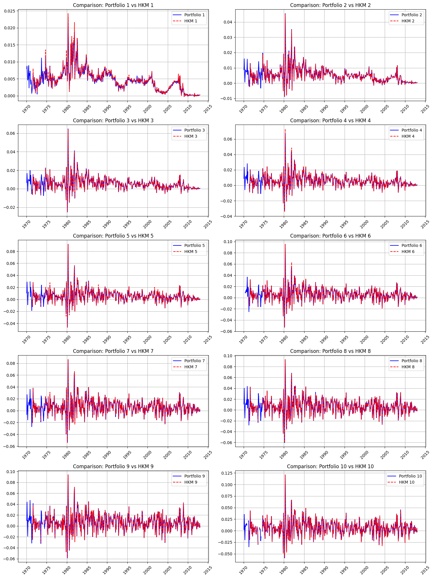
📈 Comparison of Treasury Bond Portfolio Returns: FTSFR Portfolios vs. HKM Portfolios#
The figure above compares the time-series returns of Treasury bond portfolios:
Portfolios 1–10 (in blue): Portfolios constructed by FTSFR, where Treasury bonds are sorted by time remaining to maturity, in 6-month intervals:
Portfolio 1: 0 to 6 months
Portfolio 2: 6 months to 1 year
Portfolio 3: 1 year to 1.5 years
Portfolio 4: 1.5 to 2 years
Portfolio 5: 2 to 2.5 years
Portfolio 6: 2.5 to 3 years
Portfolio 7: 3 to 3.5 years
Portfolio 8: 3.5 to 4 years
Portfolio 9: 4 to 4.5 years
Portfolio 10: 4.5 to 5 years
HKM Portfolios 1–10 (in red): Portfolios from He, Kelly, and Manella (HKM) using a similar 6-month maturity bucket structure for comparison.
🔍 Observations#
The returns between FTSFR portfolios (blue) and HKM portfolios (red) show close alignment, indicating a consistent term-structure pattern across both datasets.
During periods of heightened volatility—such as the 2008 financial crisis —portfolios with longer time to maturity generally exhibit greater return sensitivity, seen consistently in both series.
Small return differences may result from:
Rounding errors due to different data sources and small values.
Missing values in the HKM data.
This comparison confirms that the FTSFR replication tracks the structure and return behavior of the HKM maturity-sorted Treasury portfolios.