Cleaning Summary: CDS Bond Basis

Paper Introduction

This construction is based upon the structure proposed by Siriwardane, Sunderam, and Wallen in Segmented Arbitrage (https://papers.ssrn.com/sol3/papers.cfm?abstract_id=3960980). The original paper studies the concept of implied arbitrage returns in many different markets. If markets were truly frictionless, we would expect there to be perfect correlation between all of the arbitrage returns. This is because efficient capital allocation would dictate that capital be spent where the best opportunity is, thus dictating the arbitrage opportunites we calculate via different product would have correlating rates as capital would be allocated to a different source if the arbitrage opportunity looks more attractive.

CDS Par Spread Returns

Spread Construction

In the following notebook, we will walk through the steps to constructing the implied arbitrage found in the CDS and corporate bond market as specified in the Appendix of the paper (https://static1.squarespace.com/static/5e29e11bb83a3f5d75beb17d/t/654d74d916f20316049a0889/1699575002123/Appendix.pdf). The authors define the CDS basis (\(CB\)) as

\[ CB_{i, t, \tau} = CDS_{i, t, \tau} - FR_{i, t, \tau} \]

where:

• \(FR_{i, t, \tau}\) = time \(t\) floating rate spread implied by a fixed-rate corporate bond issued by firm \(i\) at tenor \(\tau\)

• \(CDS_{i, t, \tau}\) = time \(t\) Credit Default Swap (CDS) par spread for firm \(i\) with tenor \(\tau\)

A negative basis implies an investor could earn a positive arbitrage profit by going long the bond and purchasing CDS protection. The investor would pay a lower par spread than the coupon of the bond itself and then receive value from the default.

The value of \(FR\) is substituted by the paper with Z-spread which we also modify in our construction. We will go into the substitution in detail later.

The value of \(CDS\) is interpolated by the authors using a cubic spline function.

Implied Risk Free Return

Given the CDS spread from above, traditional construction of a risk free rate for implied arbitrage implied the following return.

\[ rfr^{CDS}_{i, t, \tau} = y_{t, \tau} - CB_{i , t, \tau} \]

where:

• \(y_{t, \tau}\) = maturity matched treasury yield at time \(t\)

The risk free rate then can be seen as the treasury yield in addition to the basis recieved when executing the CDS basis trade (investor benefits from negative basis).

Key Filters when selecting viable data as specified in Segmented Arbitrage

1. Include only Senior Unsecured Debt issued in USD by US firms with valid ISIN

2. Include only fixed rate bonds with maturity between 1 and 10 years

3. Include only bonds with outstanding principle of at least 100,000 USD

4. Exclude putable and convertible bonds

5. Exclude bonds trading at less than half of face value

6. Include only assets on a certain date if a cubic spline of the CDS set is possible

• There must be 2 or more CDS products corresponding to a corporate bond on a certain day for parspread cubic spline to be possible

import sys
from pathlib import Path

sys.path.insert(0, "../../src")
sys.path.insert(0, "./src")

import pandas as pd
import pull_open_source_bond
import pull_wrds_markit
from merge_cds_bond import *
from process_final_product import *

from settings import config

# %load_ext autoreload
# %autoreload 2

DATA_DIR = Path(config("DATA_DIR"))

Z-Spread (Zero-Volatility Spread)

Mathematical definition

For a bond with cash-flows \(CF_t\) at times \(t=1,\dots,N\) and Treasury spot rates \(s_t\),

\[ P = \sum_{t=1}^{N} \frac{CF_t}{\bigl(1+s_t+Z\bigr)^t}. \]

The constant \(Z\) that solves this equation is the Z-spread.

Intuition

\(Z\) is the uniform extra yield added to every point on the risk-free spot curve so that the discounted cash-flows equal the bond’s dirty price \(P\). It compensates investors for credit and liquidity risk relative to Treasuries.

Link to Yield-to-Maturity

Setting the Z-spread pricing equation equal to the standard YTM equation gives

\[\sum_{t=1}^{N}\frac{CF_t}{(1+y)^t} =\sum_{t=1}^{N}\frac{CF_t}{\bigl(1+s_t+Z\bigr)^t} \tag{A1} \]

where \(y\) is the bond’s yield-to-maturity. Except for the trivial flat-curve case (\(s_t=s\)), (A1) has no algebraic solution—\(y\) or \(Z\) must be found numerically.

Continuous-Compounding Identity

Rewrite discounts as \(e^{-r t}\). With PV-weights

\[ w_t=\frac{CF_t\,e^{-(s_t+Z)t}}{P},\qquad\sum_{t}w_t=1, \]

equation (A1) yields the convenient mean-value relationship

\[ y \;=\; \sum_{t=1}^{N} w_t\,(s_t+Z)\tag{A2} \]

Thus YTM is the PV-weighted average of the spot rates plus the Z-spread.

Practical Proxy: YTM Credit Spread

Analysts often approximate \(Z\) with the credit spread

\[ \Delta y = y_{\text{bond}} - y_{\text{Treasury-DM}}, \]

where \(y_{\text{Treasury-DM}}\) is the yield on a Treasury portfolio matched to the bond’s (modified) duration.

Why it works

1. A small parallel shift \(Z\) applied to all discount rates changes price by \(-D_{\text{mod}}\;Z\). For modest spreads, this produces nearly the same price change as replacing the spot curve with a single rate shift \(\Delta y\).

2. Duration-matching the Treasury benchmark neutralises curve-shape effects, so \(\Delta y\) isolates the average extra yield attributable to credit/liquidity risk.

3. Empirically, \(\Delta y\) tracks \(Z\) closely for plain-vanilla, option-free bonds, making it a “good-enough” proxy when full spot-curve data or iterative Z-spread calculations are impractical.

Note

Z-spread is said to be populated by Markit in the CDS dataset but during the reconstruction process we found no proxy. Thus, we chose our own construction.

Data Overview

corp_bonds_data = pull_open_source_bond.load_corporate_bond_returns(
    data_dir=DATA_DIR / "cds_bond_basis"
)
red_data = pd.read_parquet(DATA_DIR / "cds_bond_basis" / "RED_and_ISIN_mapping.parquet")
cds_data = pull_wrds_markit.load_cds_data(data_dir=DATA_DIR / "cds_bond_basis")

corp_bonds_data.info()

<class 'pandas.core.frame.DataFrame'>
RangeIndex: 1572384 entries, 0 to 1572383
Data columns (total 49 columns):
 #   Column           Non-Null Count    Dtype         
---  ------           --------------    -----         
 0   date             1572384 non-null  datetime64[ns]
 1   cusip            1572384 non-null  object        
 2   issuer_cusip     1572384 non-null  object        
 3   permno           1422169 non-null  float64       
 4   exretn_t+1       1041541 non-null  float64       
 5   exretnc_bns_t+1  1030933 non-null  float64       
 6   exretnc_t+1      1038056 non-null  float64       
 7   exretnc_dur_t+1  1038056 non-null  float64       
 8   bond_ret_t+1     1041541 non-null  float64       
 9   bond_ret         1046059 non-null  float64       
 10  exretn           1046059 non-null  float64       
 11  exretnc_bns      1035383 non-null  float64       
 12  exretnc          1042538 non-null  float64       
 13  exretnc_dur      1042538 non-null  float64       
 14  rating           1398323 non-null  float64       
 15  cs               1389316 non-null  float64       
 16  cs_6m_delta      1200967 non-null  float64       
 17  bond_yield       1389838 non-null  float64       
 18  bond_amount_out  1398323 non-null  float64       
 19  offering_amt     1398323 non-null  float64       
 20  bondprc          1188065 non-null  float64       
 21  perc_par         1188065 non-null  float64       
 22  tmt              1398323 non-null  float64       
 23  duration         1389316 non-null  float64       
 24  ind_num_17       1036811 non-null  float64       
 25  sic_code         1398323 non-null  float64       
 26  mom6_1           1468700 non-null  float64       
 27  ltrev48_12       770557 non-null   float64       
 28  BOND_RET         1206499 non-null  float64       
 29  ILLIQ            1137969 non-null  float64       
 30  var95            672058 non-null   float64       
 31  n_trades_month   1212316 non-null  float64       
 32  size_ig          1398323 non-null  float64       
 33  size_jk          1398323 non-null  float64       
 34  zcb              1398323 non-null  float64       
 35  conv             1398323 non-null  float64       
 36  BOND_YIELD       1294588 non-null  float64       
 37  CS               1294588 non-null  float64       
 38  BONDPRC          1294588 non-null  float64       
 39  PRFULL           1294588 non-null  float64       
 40  DURATION         1294588 non-null  float64       
 41  CONVEXITY        1294588 non-null  float64       
 42  CS_6M_DELTA      1084920 non-null  float64       
 43  bond_value       1188065 non-null  float64       
 44  BOND_VALUE       1294585 non-null  float64       
 45  coupon           1572384 non-null  float64       
 46  bond_type        1572384 non-null  object        
 47  principal_amt    1572384 non-null  float64       
 48  bondpar_mil      1398323 non-null  float64       
dtypes: datetime64[ns](1), float64(45), object(3)
memory usage: 587.8+ MB

As a proxy for the Z-spread, we will use the credit spread between the bond’s yield and the yield on a Treasury portfolio matched to the bond’s (modified) duration. In this data,

• “cs” is the market-microstructure-noise-biased credit spread

• “CS” is the credit spread that has been adjusted for the market-microstructure noise. We will use this as our proxy for the Z-spread.

• “BOND_YIELD” is the corporate bond yield that has been adjusted for market-microstructure noise. We will use “BOND_YIELD” - “CS” as our treasury yield during the period.

corp_bonds_data.describe()

	date	permno	exretn_t+1	exretnc_bns_t+1	exretnc_t+1	exretnc_dur_t+1	bond_ret_t+1	bond_ret	exretn	exretnc_bns	...	BONDPRC	PRFULL	DURATION	CONVEXITY	CS_6M_DELTA	bond_value	BOND_VALUE	coupon	principal_amt	bondpar_mil
count	1572384	1.422169e+06	1.041541e+06	1.030933e+06	1.038056e+06	1.038056e+06	1.041541e+06	1.046059e+06	1.046059e+06	1.035383e+06	...	1.294588e+06	1.294588e+06	1.294588e+06	1.294588e+06	1.084920e+06	1.188065e+06	1.294585e+06	1.572384e+06	1.572384e+06	1.398323e+06
mean	2013-03-05 13:07:44.259111936	5.166780e+04	3.282121e-03	2.130163e-03	2.326617e-03	2.529531e-03	4.099201e-03	4.168516e-03	3.349400e-03	2.137542e-03	...	1.050217e+02	1.063816e+02	6.507442e+00	8.344123e+01	-3.073578e-02	6.512686e+07	6.196192e+07	5.730033e+00	9.998092e+02	5.559556e+02
min	2002-08-31 00:00:00	1.002500e+04	-9.767108e-01	-9.788410e-01	-9.754962e-01	-9.750838e-01	-9.753108e-01	-9.753108e-01	-9.767108e-01	-9.788410e-01	...	1.000000e-04	1.009944e-01	5.683952e-03	1.021010e-04	-1.066395e+01	1.500000e+01	1.700000e+01	0.000000e+00	1.000000e+01	1.000000e-03
25%	2007-12-31 00:00:00	2.322900e+04	-6.494539e-03	-5.660667e-03	-6.013460e-03	-5.673846e-03	-5.630089e-03	-5.611824e-03	-6.479160e-03	-5.682974e-03	...	9.967818e+01	1.005404e+02	3.231727e+00	1.276730e+01	-2.339199e-01	2.726895e+07	2.593350e+07	4.200000e+00	1.000000e+03	2.386430e+02
50%	2013-07-31 00:00:00	5.627400e+04	2.460858e-03	1.367245e-03	1.515543e-03	1.514050e-03	3.312874e-03	3.337704e-03	2.483598e-03	1.364946e-03	...	1.042477e+02	1.055880e+02	5.275024e+00	3.381145e+01	-4.462923e-02	4.723913e+07	4.368532e+07	5.875000e+00	1.000000e+03	4.000000e+02
75%	2018-04-30 00:00:00	7.892700e+04	1.359472e-02	1.012049e-02	1.096072e-02	1.054284e-02	1.441620e-02	1.448506e-02	1.366403e-02	1.013573e-02	...	1.105670e+02	1.121482e+02	8.567085e+00	9.504011e+01	1.521478e-01	7.836473e+07	7.508250e+07	7.125000e+00	1.000000e+03	7.000000e+02
max	2022-09-30 00:00:00	9.343300e+04	3.683310e+00	3.679218e+00	1.093704e+00	1.026469e+00	3.683510e+00	3.683510e+00	3.683310e+00	3.679218e+00	...	8.491486e+03	8.491486e+03	3.546374e+01	1.346690e+03	7.585604e+00	1.899989e+09	1.908028e+09	1.650000e+01	1.000000e+03	1.500000e+04
std	NaN	2.817581e+04	4.198366e-02	4.125521e-02	4.183619e-02	4.056453e-02	4.193871e-02	4.217267e-02	4.221634e-02	4.147882e-02	...	1.604661e+01	1.615361e+01	4.342256e+00	1.118131e+02	4.059461e-01	6.674075e+07	6.490551e+07	2.133292e+00	1.374154e+01	5.971824e+02

8 rows × 46 columns

Step 1: Merge the Redcodes of firms on to the corporate bonds.

The code for it is in merge_cds_bond.py in the function merge_redcode_into_bond_treas. The more specific inputs are within the function itself.

Given CDS tables record issuers of the Credit Default Swaps using Redcode and the bond tables only had CUSIPs, we needed to conduct a merge using a redcode-CUSIP matching table to the end product of step 1.2 for CDS processing later on.

We will pull the results without processing for CDS implied arbitrage returns.

corp_red_data = merge_red_code_into_bond_treas(corp_bonds_data, red_data)

corp_red_data.head()

	date	cusip	issuer_cusip	BOND_YIELD	CS	size_ig	size_jk	mat_days	redcode
0	2013-05-31	00101JAE6	00101J	0.021252	0.013751	1.0	1.0	1506.0	0A119O
1	2013-05-31	00101JAE6	00101J	0.021252	0.013751	1.0	1.0	1506.0	UU079R
2	2013-06-30	00101JAE6	00101J	0.026850	0.017144	1.0	1.0	1476.0	0A119O
3	2013-06-30	00101JAE6	00101J	0.026850	0.017144	1.0	1.0	1476.0	UU079R
4	2013-07-31	00101JAE6	00101J	0.023579	0.014047	1.0	1.0	1445.0	0A119O

corp_red_data.describe()

	date	BOND_YIELD	CS	size_ig	size_jk	mat_days
count	1398784	1.252264e+06	1.252264e+06	1.316230e+06	1.316230e+06	1.316230e+06
mean	2013-01-17 01:58:03.485084672	4.866752e-02	2.608657e-02	8.228288e-01	9.783617e-01	3.761267e+03
min	2002-08-31 00:00:00	-7.918977e-01	-8.427172e-01	0.000000e+00	0.000000e+00	3.610000e+02
25%	2008-01-31 00:00:00	2.911486e-02	9.941452e-03	1.000000e+00	1.000000e+00	1.342000e+03
50%	2013-03-31 00:00:00	4.339818e-02	1.698669e-02	1.000000e+00	1.000000e+00	2.479000e+03
75%	2018-01-31 00:00:00	5.791579e-02	2.852355e-02	1.000000e+00	1.000000e+00	5.522000e+03
max	2022-09-30 00:00:00	2.442612e+01	2.441472e+01	1.000000e+00	1.000000e+00	3.652500e+04
std	NaN	6.505191e-02	6.460367e-02	3.818136e-01	1.454995e-01	3.532676e+03

Step 2: CDS data pull and CDS data processing

Step 2.1: CDS data pull

The CDS data pull will be filtered using the redcodes from the above bond_redcode_merged_data dataframe, ensuring that only the firms that have corporate bond data are pulled from the CDS table. Daily CDS data is being pulled initially,

resulting in a mismatch in amount compared to corporate bonds. The data will be reduced during the merge process as the corporate bonds are indicated by monthly data.

Step 2.2: CDS data processing

Let’s first observe the data to see what we are working with:

cds_data.info()

<class 'pandas.core.frame.DataFrame'>
RangeIndex: 46851870 entries, 0 to 46851869
Data columns (total 7 columns):
 #   Column     Dtype         
---  ------     -----         
 0   date       datetime64[ns]
 1   ticker     string        
 2   redcode    string        
 3   parspread  Float64       
 4   tenor      string        
 5   country    string        
 6   year       int64         
dtypes: Float64(1), datetime64[ns](1), int64(1), string(4)
memory usage: 2.5 GB

cds_data.describe()

	date	parspread	year
count	46851870	46707717.0	4.685187e+07
mean	2011-12-19 02:04:52.993115392	0.021868	2.011462e+03
min	2001-01-02 00:00:00	0.000007	2.001000e+03
25%	2006-12-18 00:00:00	0.003602	2.006000e+03
50%	2010-07-13 00:00:00	0.007839	2.010000e+03
75%	2017-05-02 00:00:00	0.018148	2.017000e+03
max	2023-12-29 00:00:00	491.842763	2.023000e+03
std	NaN	0.638027	6.115298e+00

The CDS data has a flaw: the tenor is displayed as opposed to maturity date which would allow for more accurate cubic splines of the par spread. To approximate the correct number of days, we use tenor as is and annualize.

For example, if the tenor is \(3Y\), the number of days that we use to annualize is \(3 \times 365 = 1095\).

In our processing function merge_cds_bond, we grab the redcode, date tuples for which we can generate a viable cubic spline function, filter the bond and treasury dataframe (output of step 1).

Then, we use the days between the maturity and the date for each corporate bond as the input for the cubic spline function for par spread generation. Thus, our final product contains corporate bonds, duration matched treasury rates, and implied

CDS par spreads as specified by the Segmented Arbitrage paper.

final_data = merge_cds_into_bonds(corp_red_data, cds_data)

final_data.head()

	cusip	date	mat_days	BOND_YIELD	CS	size_ig	size_jk	par_spread
39	00101JAE6	2014-12-31	927.0	0.033902	0.025627	1.0	1.0	0.034591
45	00101JAE6	2015-03-31	837.0	0.026494	0.020114	1.0	1.0	0.017713
47	00101JAE6	2015-04-30	807.0	0.024420	0.018444	1.0	1.0	0.017103
51	00101JAE6	2015-06-30	746.0	0.026136	0.019872	1.0	1.0	0.016516
53	00101JAE6	2015-07-31	715.0	0.022742	0.015899	1.0	1.0	0.012640

Step 3: Processing

Revisiting the original model:

\[ CB_{i, t, \tau} = CDS_{i, t, \tau} - FR_{i, t, \tau} \]

where:

• \(FR_{i, t, \tau}\) = time \(t\) floating rate spread implied by a fixed-rate corporate bond issued by firm \(i\) at tenor \(\tau\)

  • We use “CS” from the original corporate bonds table for this

• \(CDS_{i, t, \tau}\) = time \(t\) Credit Default Swap (CDS) par spread for firm \(i\) with tenor \(\tau\)

  • CDS parspread is constructed using a Cubic Spline

\[ rfr^{CDS}_{i, t, \tau} = y_{t, \tau} - CB_{i , t, \tau} \]

where:

• \(y_{t, \tau}\) = duration matched treasury yield at time \(t\)

  • this is constructed via the “BOND_YIELD” - “CS” in the original corporate bond table

Note: Filtering

We threw out some unreasonable data for the absolute rf values exceeding 1 (risk free annual return of 100%).

processed_final_data = process_cb_spread(final_data)

processed_final_data.head()

	cusip	date	mat_days	BOND_YIELD	CS	size_ig	size_jk	par_spread	FR	CB	rfr	c_rating
39	00101JAE6	2014-12-31	927.0	0.033902	0.025627	1.0	1.0	0.034591	0.025627	0.008964	-0.068971	IG + HY
45	00101JAE6	2015-03-31	837.0	0.026494	0.020114	1.0	1.0	0.017713	0.020114	-0.002401	0.878103	IG + HY
47	00101JAE6	2015-04-30	807.0	0.024420	0.018444	1.0	1.0	0.017103	0.018444	-0.001340	0.731656	IG + HY
51	00101JAE6	2015-06-30	746.0	0.026136	0.019872	1.0	1.0	0.016516	0.019872	-0.003356	0.961969	IG + HY
53	00101JAE6	2015-07-31	715.0	0.022742	0.015899	1.0	1.0	0.012640	0.015899	-0.003259	1.010164	IG + HY

processed_final_data.info()

<class 'pandas.core.frame.DataFrame'>
Index: 585507 entries, 39 to 1398297
Data columns (total 12 columns):
 #   Column      Non-Null Count   Dtype         
---  ------      --------------   -----         
 0   cusip       585507 non-null  object        
 1   date        585507 non-null  datetime64[ns]
 2   mat_days    585507 non-null  float64       
 3   BOND_YIELD  585507 non-null  float64       
 4   CS          585507 non-null  float64       
 5   size_ig     585507 non-null  float64       
 6   size_jk     585507 non-null  float64       
 7   par_spread  585507 non-null  float64       
 8   FR          585507 non-null  float64       
 9   CB          585507 non-null  float64       
 10  rfr         585507 non-null  float64       
 11  c_rating    585507 non-null  object        
dtypes: datetime64[ns](1), float64(9), object(2)
memory usage: 58.1+ MB

processed_final_data.describe()

	date	mat_days	BOND_YIELD	CS	size_ig	size_jk	par_spread	FR	CB	rfr
count	585507	585507.000000	585507.000000	585507.000000	585507.000000	585507.000000	585507.000000	585507.000000	585507.000000	585507.000000
mean	2013-08-09 15:05:17.429509632	3639.666931	0.045777	0.023430	0.849758	0.981083	0.023292	0.023430	-0.000138	2.248486
min	2002-09-30 00:00:00	361.000000	-0.791898	-0.842717	0.000000	0.000000	-0.964251	-0.842717	-0.981998	-99.986240
25%	2008-10-31 00:00:00	1320.000000	0.027924	0.009315	1.000000	1.000000	0.002744	0.009315	-0.012180	1.343552
50%	2013-12-31 00:00:00	2419.000000	0.041776	0.015993	1.000000	1.000000	0.007503	0.015993	-0.005046	2.579079
75%	2018-05-31 00:00:00	5281.000000	0.056008	0.026505	1.000000	1.000000	0.020888	0.026505	-0.001138	4.404756
max	2022-09-30 00:00:00	36478.000000	5.665780	5.663980	1.000000	1.000000	5.728639	5.663980	1.043381	99.845030
std	NaN	3182.769546	0.041844	0.040593	0.357309	0.136232	0.111905	0.040593	0.104321	10.388473

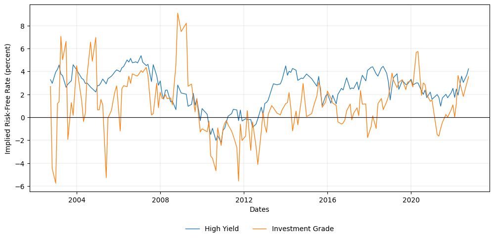
Step 4: Results

Below is a graph of 3 categories of bonds where certain ETFs may include both IG and Junk (HY) bonds.

Rating 0: Only junk bonds (HY)

Rating 1: Only IG bonds

Rating 2: Both IG and Junk bonds (HY) in the product

generate_graph(processed_final_data)