Imports

import sys

sys.path.insert(1, "./../")

import numpy as np
import pandas as pd
import seaborn as sns
import matplotlib.pyplot as plt

from pathlib import Path

from settings import config
from datetime import date
import warnings
from scipy.stats import norm, stats

from scipy import stats

from scipy.stats import shapiro, jarque_bera, normaltest, skew, kurtosis

import plotly.io as pio

pio.templates.default = "plotly_white"
warnings.filterwarnings("ignore")

OUTPUT_DIR = Path(config("OUTPUT_DIR"))
DATA_DIR = Path(config("DATA_DIR"))
WRDS_USERNAME = config("WRDS_USERNAME")

START_DATE_01 = date(1996, 1, 1)
END_DATE_01 = date(2012, 1, 31)

START_DATE_02 = date(2012, 2, 1)
END_DATE_02 = date(2024, 12, 31)

DATE_RANGE = f"{pd.Timestamp(START_DATE_01):%Y-%m}_{pd.Timestamp(END_DATE_02):%Y-%m}"

Functions

# --- Black-Scholes elasticity ---
def bs_elasticity(S, K, T, r, sigma, option_type="call"):
    d1 = (np.log(S / K) + (r + 0.5 * sigma**2) * T) / (sigma * np.sqrt(T))
    if option_type == "call":
        price = S * norm.cdf(d1) - K * np.exp(-r * T) * norm.cdf(
            d1 - sigma * np.sqrt(T)
        )
        delta = norm.cdf(d1)
    else:
        price = K * np.exp(-r * T) * norm.cdf(-d1 + sigma * np.sqrt(T)) - S * norm.cdf(
            -d1
        )
        delta = -norm.cdf(-d1)
    return (delta * S / price), price


# Gaussian kernel function
def kernel_weights(m_grid, ttm_grid, k_s, ttm, bw_m=0.0125, bw_t=10):
    m_grid = np.asarray(m_grid, dtype=float)
    ttm_grid = np.asarray(ttm_grid, dtype=float)
    x = (m_grid - k_s) / bw_m
    y = (ttm_grid - ttm) / bw_t
    dist_sq = x**2 + y**2
    weights = np.exp(-0.5 * dist_sq)
    return weights / weights.sum() if weights.sum() > 0 else np.zeros_like(weights)


# --- Construct a single day portfolio ---
def construct_portfolio(data, k_s_target, ttm_target, option_type="call", r=0.01):
    subset = data[(data["option_type"] == option_type)]
    weights = kernel_weights(subset["moneyness"], subset["ttm"], k_s_target, ttm_target)
    subset = subset.assign(weight=weights)
    subset = subset[subset["weight"] > 0.01]
    subset["weight"] /= subset["weight"].sum()

    # Leverage-adjusted returns
    elast, price = bs_elasticity(
        S=subset["underlying"],
        K=subset["strike"],
        T=subset["ttm"] / 365,
        r=r,
        sigma=subset["iv"],
        option_type=option_type,
    )
    subset["leverage_return"] = subset["daily_return"] / elast

    return (subset["leverage_return"] * subset["weight"]).sum()


# --- Main Loop (simplified) ---
def build_portfolios(option_data, m_grid, ttm_grid, option_types=["call", "put"]):
    portfolios = []
    for opt_type in option_types:
        for k_s in m_grid:
            for ttm in ttm_grid:
                ret = construct_portfolio(option_data, k_s, ttm, option_type=opt_type)
                portfolios.append(
                    {"type": opt_type, "moneyness": k_s, "ttm": ttm, "return": ret}
                )
    return pd.DataFrame(portfolios)


def calc_kernel_weights(spx_mod):
    """Calculate kernel weights for each option in the SPX dataset based on moneyness and maturity targets.
    This function iterates through predefined moneyness and maturity targets, applies kernel weights to candidate options."""

    # Define moneyness and maturity targets from the paper
    moneyness_targets = [0.90, 0.925, 0.950, 0.975, 1.000, 1.025, 1.050, 1.075, 1.100]
    maturity_targets = [30, 60, 90]
    cp_flags = ["C", "P"]

    # Preprocess base DataFrame
    spx_mod["days_to_maturity_int"] = spx_mod["days_to_maturity"].dt.days
    spx_mod = spx_mod.reset_index()
    spx_mod["original_index"] = spx_mod.index

    weight_results = []

    # Iterate through each strategy target
    for cp_flag in cp_flags:
        for target_moneyness in moneyness_targets:
            for target_ttm in maturity_targets:
                # Filter candidate options
                candidate_options = spx_mod[
                    (spx_mod["cp_flag"] == cp_flag)
                    & (spx_mod["moneyness_id"] == target_moneyness)
                    & (spx_mod["maturity_id"] == target_ttm)
                ].copy()

                if candidate_options.empty:
                    continue

                candidate_options["kernel_weight"] = np.nan

                # Apply kernel weights per date
                for date, g in candidate_options.groupby("date"):
                    idx = g.index
                    weights = kernel_weights(
                        g["moneyness"].values,
                        g["days_to_maturity_int"].values,
                        k_s=target_moneyness,
                        ttm=target_ttm,
                    )
                    candidate_options.loc[idx, "kernel_weight"] = weights

                weight_results.append(
                    candidate_options[["original_index", "kernel_weight"]]
                )

    # Merge weights back into spx_mod
    if weight_results:
        all_weights = pd.concat(weight_results).set_index("original_index")
        spx_mod.set_index("original_index", inplace=True)
        spx_mod["kernel_weight"] = all_weights["kernel_weight"]
        spx_mod.reset_index(inplace=True)
    else:
        print("No matching options found for any target.")

    spx_mod.drop(columns=["original_index"], inplace=True)
    return spx_mod

def calc_option_delta_elasticity(df):
    df = df.copy()

    T = df["days_to_maturity"].dt.days / 365.0
    S = df["close"]
    K = df["strike_price"]
    r = df["tb_m3"] / 100
    sigma = df["IV"]
    d1 = (np.log(S / K) + (r + 0.5 * sigma**2) * T) / (sigma * np.sqrt(T))

    df = df.assign(
        option_delta=np.where(df["cp_flag"] == "C", norm.cdf(d1), norm.cdf(d1) - 1),
        option_elasticity=lambda x: x["option_delta"] * x["close"] / x["mid_price"],
    )

    return df

def read_option_data(filename):
    # Example string interval: '(0.9, 0.95]'
    # Remove whitespace and parse the string into tuples
    def parse_interval_string(s):
        # Handle missing or malformed entries gracefully
        if pd.isnull(s) or not isinstance(s, str):
            return pd.NA  # or np.nan
        s = s.strip().replace("(", "").replace("]", "")
        try:
            left, right = map(float, s.split(","))
            return pd.Interval(left, right, closed="right")
        except ValueError:
            return pd.NA

    df = pd.read_parquet(filename)

    # restore the 'moneyness_bin' column as intervals
    df["moneyness_bin"] = df["moneyness_bin"].apply(parse_interval_string)

    return df

def compute_cjs_return_leverage_investment(spx_mod):
    df = spx_mod.copy()
    df = df.sort_values(["ftfsa_id", "date"])

    # Lag price
    df["mid_price_lag"] = df.groupby("ftfsa_id")["mid_price"].shift(1)

    # Return and daily risk-free rate
    df["option_return"] = (df["mid_price"] - df["mid_price_lag"]) / df["mid_price_lag"]
    df["daily_rf"] = df["tb_m3"] / 100 / 252

    # Weighted dollar investment and return contribution
    df["inv_weight"] = df["kernel_weight"] / df["option_elasticity"]
    df["inv_return"] = df["inv_weight"] * df["option_return"]

    # Group and aggregate
    grouped = df.groupby(["date", "ftfsa_id"])

    port = grouped.agg(
        total_inv_weight=("inv_weight", "sum"),
        total_inv_return=("inv_return", "sum"),
        daily_rf=("daily_rf", "first"),
        cp_flag=("cp_flag", "first"),
    ).reset_index()

    # Apply CJS logic
    def adjusted_return(row):
        if row["cp_flag"] == "C":
            return (
                row["total_inv_return"]
                + (1 - row["total_inv_weight"]) * row["daily_rf"]
            )
        elif row["cp_flag"] == "P":
            return (
                -row["total_inv_return"]
                + (1 + row["total_inv_weight"]) * row["daily_rf"]
            )
        else:
            return np.nan

    port["portfolio_return"] = port.apply(adjusted_return, axis=1)

    return port

# Function to compute normality metrics
def normality_summary(df):
    summary = []
    for col in df.columns:
        series = df[col].dropna()
        shapiro_p = shapiro(series)[1]
        jb_stat, jb_p = jarque_bera(series)
        normaltest_p = normaltest(series)[1]
        skew_val = skew(series)
        kurt_val = kurtosis(series, fisher=False)
        summary.append(
            {
                "Series": col,
                "Shapiro_p": shapiro_p,
                "JarqueBera_p": jb_p,
                "Normaltest_p": normaltest_p,
                "Skewness": skew_val,
                "Kurtosis": kurt_val,
            }
        )
    return pd.DataFrame(summary)

Execution

# read filtered data
source_file = Path(DATA_DIR / "options" / f"spx_filtered_final_{DATE_RANGE}.parquet")
spx_filtered = read_option_data(filename=source_file)
spx_filtered = spx_filtered.reset_index()

# create the moneyness ID from the moneyness_bin column, using the right edge of the interval
spx_filtered["moneyness_id"] = spx_filtered["moneyness_bin"].apply(
    lambda x: x.right if pd.notnull(x) else np.nan
)
# drop any rows where moneyness_id is NaN
spx_filtered = spx_filtered.dropna(subset=["moneyness_id"])

spx_filtered

	date	exdate	moneyness	secid	open	close	cp_flag	IV	tb_m3	volume	...	days_to_maturity	pc_parity_int_rate	intrinsic	log_iv	fitted_iv	rel_distance_iv	moneyness_bin	stdev_iv_moneyness_bin	is_outlier_iv	moneyness_id
0	1996-01-04	1996-01-20	0.987534	108105.0	621.32	617.70	C	0.082711	5.04	444.0	...	16 days	0.015898	7.70	-2.492403	-2.377298	4.841838	(0.975, 1.0]	3.516840	False	1.000
1	1996-01-04	1996-01-20	1.019913	108105.0	621.32	617.70	C	0.097356	5.04	4022.0	...	16 days	0.015898	0.00	-2.329381	-2.285771	1.907866	(1.0, 1.025]	5.219336	False	1.025
2	1996-01-04	1996-01-20	1.028007	108105.0	621.32	617.70	C	0.101756	5.04	1627.0	...	16 days	0.015898	0.00	-2.285177	-2.264082	0.931727	(1.025, 1.05]	4.396845	False	1.050
3	1996-01-04	1996-01-20	1.036102	108105.0	621.32	617.70	C	0.100588	5.04	0.0	...	16 days	0.015898	0.00	-2.296722	-2.242870	2.401027	(1.025, 1.05]	4.396845	False	1.050
4	1996-01-04	1996-02-17	0.963251	108105.0	621.32	617.70	C	0.071852	5.04	3.0	...	44 days	0.014622	22.70	-2.633147	-2.563785	2.705450	(0.95, 0.975]	2.301503	False	0.975
...	...	...	...	...	...	...	...	...	...	...	...	...	...	...	...	...	...	...	...	...	...
3195881	2019-12-31	2020-06-19	1.044639	108105.0	3215.18	3230.78	P	0.117063	1.52	0.0	...	171 days	0.014769	144.22	-2.145043	-2.132215	0.601630	(1.025, 1.05]	4.396845	False	1.050
3195882	2019-12-31	2020-06-19	1.052377	108105.0	3215.18	3230.78	P	0.113900	1.52	0.0	...	171 days	0.014769	169.22	-2.172434	-2.165558	0.317525	(1.05, 1.075]	5.236635	False	1.075
3195883	2019-12-31	2020-06-19	1.060116	108105.0	3215.18	3230.78	P	0.110925	1.52	20.0	...	171 days	0.014769	194.22	-2.198901	-2.199596	-0.031616	(1.05, 1.075]	5.236635	False	1.075
3195884	2019-12-31	2020-06-19	1.067854	108105.0	3215.18	3230.78	P	0.108540	1.52	0.0	...	171 days	0.014769	219.22	-2.220637	-2.234330	-0.612848	(1.05, 1.075]	5.236635	False	1.075
3195885	2019-12-31	2020-06-19	1.075592	108105.0	3215.18	3230.78	P	0.106814	1.52	0.0	...	171 days	0.014769	244.22	-2.236666	-2.269758	-1.457925	(1.075, 1.1]	5.723928	False	1.100

2676696 rows × 26 columns

Construction of Monthly Leverage-Adjusted Portfolio Returns in CJS

Process

The construction of the 27 call and 27 put portfolios in CJS is a multi-step process, with the objective of developing portfolio returns series that are stationary and only moderately skewed. Note that the discrete bucketing of moneyness and days to maturity lead to multiple candidate options for each portfolio on each trading day. These options are given weights according to a bivariate Gaussian weighting kernel in moneyness and maturity (bandwidths: 0.0125 in moneyness and 10 days to maturity).

Each portfolio’s daily returns are initially calculated as simple arithmetic return, assuming the option is bought and sold at its bid-ask midpoint at each rebalancing. The one-day arithmetic return is then converted to a leverage-adjusted return. This procedure is achieved by calculating the one-day return of a hypothetical portfolio with \(\omega_{BSM}^{-1}\) dollars invested in the option, and \((1 - \omega^{-1})\) dollars invested in the risk-free rate, where \(\omega_{BSM}\) is the BSM elasticity based on the implied volatility of the option.

(1)\[\begin{align} \omega_{\text{BSM, Call}} &= \frac{\partial C_{\text{BSM}}}{\partial S} \cdot \frac{S}{C_{\text{BSM}}} > 1 \\ \omega_{\text{BSM, Put}} &= \frac{\partial P_{\text{BSM}}}{\partial S} \cdot \frac{S}{P_{\text{BSM}}} < -1 \end{align}\]

Each leverage-adjusted call portfolio comprises of a long position in a fraction of a call, and some investment in the risk-free rate.

Each leverage-adjusted put portfolio comprises of a short position in a fraction of a put, and >100% investment in the risk-free rate.

For clarity, we present below the mathematics behind CJS’ descriptions of the portfolio construction process. The following applies for a single trading day \(t\), for a set of candidate call or put options. Portfolios in CJS are identified by 3 characteristics: option type (call or put), moneyness (9 discrete targets), and time to maturity (3 discrete targets). On any given day, it is rare to find options that exactly match the moneyness and maturity targets. Instead, there may be multiple options that are “close to” the target moneyness / maturity (each a “candidate option”). Furthermore, each candidate option has its own price and price sensitivity to changes in the underlying SPX index level. In order to arrive at a “price” for an option portfolio, CJS applies a Gaussian weighting kernel in moneyness and maturity, as described below. This kernel-weighted price across the candidate options on a given day is used as the price of the option component of the portfolio (the other component being the risk-free rate). This portfolio is leverage-adjusted using the BSM elasticity, in order to standardize the sensitivity of OTM and ITM portfolios to changes in the underlying.

1. Gaussian Kernel Weighting

Let:

• \(m_{i}\) = moneyness of option \(i\)

• \(\tau_{i}\) = days to maturity of option \(i\)

• \(k_{s}\) = target moneyness

• \(\tau\) = target maturity

• \(h_{m}\), \(h_{\tau}\) = bandwidths for moneyness and maturity

• \(d_{i}^2 = \left( \frac{m_{i} - k_{s}}{h_{m}} \right)^2 + \left( \frac{\tau_{i} - \tau}{h_{\tau}} \right)^2\)

Then the unnormalized Gaussian weight for option \(i\) is:

\[ w_{i}^* = \exp\left( -\frac{1}{2} d_{i}^2 \right) \]

The normalized kernel weight:

\[ w_{i} = \frac{w_{i}^*}{\sum_j w_j^*} \]

---

2. Option Elasticity

Let:

• \(S_{t}\) = underlying index level at time \(t\)

• \(P_{i}\) = price of option \(i\)

• \(\Delta_{i}\) = option delta

Then:

\[ \varepsilon_{i} = \frac{S_t \cdot \Delta_{i}}{P_{i}} \]

---

3. Arithmetic Return of Option \(i\)

Let:

• \(P_{i,t-1}\) = price of option \(i\) at time \(t-1\)

• \(P_{i,t}\) = price of option \(i\) at time \(t\)

Then:

\[ r_{i} = \frac{P_{i,t} - P_{i,t-1}}{P_{i,t-1}} \]

---

4. Leverage-Adjusted Portfolio Construction

Let:

• \(r_{f}\) = risk-free rate on day \(t\)

The leverage-adjusted return of the call portfolio is:

\[ R_t^{call} = \sum_{i} w_{i} \cdot \frac{1}{\varepsilon_{i}} \cdot r_{i} + \left(1 - \sum_{i} w_{i} \cdot \frac{1}{\varepsilon_{i}} \right) \cdot r_f \]

The leverage-adjusted return of the put portfolio is:

\[ R_t^{put} = -\sum_{i} w_{i} \cdot \frac{1}{\varepsilon_{i}} \cdot r_{i} + \left(1 + \sum_{i} w_{i} \cdot \frac{1}{\varepsilon_{i}} \right) \cdot r_f \]

Below we implement this process.

Implementation

1. Build the FTSFA ID for each portfolio

# identify the maturity ID based on the closest maturity to 30, 60, or 90 days
maturity_id = pd.concat(
    (
        abs(spx_filtered["days_to_maturity"].dt.days - 30),
        abs(spx_filtered["days_to_maturity"].dt.days - 60),
        abs(spx_filtered["days_to_maturity"].dt.days - 90),
    ),
    axis=1,
)
maturity_id.columns = [30, 60, 90]
spx_filtered["maturity_id"] = maturity_id.idxmin(axis=1)
spx_filtered["ftfsa_id"] = (
    spx_filtered["cp_flag"]
    + "_"
    + (spx_filtered["moneyness_id"] * 1000).apply(
        lambda x: str(int(x)) if pd.notnull(x) and x == int(x) else str(x)
    )
    + "_"
    + spx_filtered["maturity_id"].astype(str)
)

# set index to ftfsa_id and date
spx_filtered.set_index(["ftfsa_id", "date"], inplace=True)
spx_filtered

		exdate	moneyness	secid	open	close	cp_flag	IV	tb_m3	volume	open_interest	...	pc_parity_int_rate	intrinsic	log_iv	fitted_iv	rel_distance_iv	moneyness_bin	stdev_iv_moneyness_bin	is_outlier_iv	moneyness_id	maturity_id
ftfsa_id	date
C_1000_30	1996-01-04	1996-01-20	0.987534	108105.0	621.32	617.70	C	0.082711	5.04	444.0	5905.0	...	0.015898	7.70	-2.492403	-2.377298	4.841838	(0.975, 1.0]	3.516840	False	1.000	30
C_1025_30	1996-01-04	1996-01-20	1.019913	108105.0	621.32	617.70	C	0.097356	5.04	4022.0	5969.0	...	0.015898	0.00	-2.329381	-2.285771	1.907866	(1.0, 1.025]	5.219336	False	1.025	30
C_1050_30	1996-01-04	1996-01-20	1.028007	108105.0	621.32	617.70	C	0.101756	5.04	1627.0	6224.0	...	0.015898	0.00	-2.285177	-2.264082	0.931727	(1.025, 1.05]	4.396845	False	1.050	30
	1996-01-04	1996-01-20	1.036102	108105.0	621.32	617.70	C	0.100588	5.04	0.0	6593.0	...	0.015898	0.00	-2.296722	-2.242870	2.401027	(1.025, 1.05]	4.396845	False	1.050	30
C_975_30	1996-01-04	1996-02-17	0.963251	108105.0	621.32	617.70	C	0.071852	5.04	3.0	34.0	...	0.014622	22.70	-2.633147	-2.563785	2.705450	(0.95, 0.975]	2.301503	False	0.975	30
...	...	...	...	...	...	...	...	...	...	...	...	...	...	...	...	...	...	...	...	...	...	...
P_1050_90	2019-12-31	2020-06-19	1.044639	108105.0	3215.18	3230.78	P	0.117063	1.52	0.0	395.0	...	0.014769	144.22	-2.145043	-2.132215	0.601630	(1.025, 1.05]	4.396845	False	1.050	90
P_1075_90	2019-12-31	2020-06-19	1.052377	108105.0	3215.18	3230.78	P	0.113900	1.52	0.0	163.0	...	0.014769	169.22	-2.172434	-2.165558	0.317525	(1.05, 1.075]	5.236635	False	1.075	90
	2019-12-31	2020-06-19	1.060116	108105.0	3215.18	3230.78	P	0.110925	1.52	20.0	310.0	...	0.014769	194.22	-2.198901	-2.199596	-0.031616	(1.05, 1.075]	5.236635	False	1.075	90
	2019-12-31	2020-06-19	1.067854	108105.0	3215.18	3230.78	P	0.108540	1.52	0.0	12.0	...	0.014769	219.22	-2.220637	-2.234330	-0.612848	(1.05, 1.075]	5.236635	False	1.075	90
P_1100_90	2019-12-31	2020-06-19	1.075592	108105.0	3215.18	3230.78	P	0.106814	1.52	0.0	0.0	...	0.014769	244.22	-2.236666	-2.269758	-1.457925	(1.075, 1.1]	5.723928	False	1.100	90

2676696 rows × 26 columns

portfolio_ids = spx_filtered.index.get_level_values("ftfsa_id").unique()
portfolio_ids

Index(['C_1000_30', 'C_1025_30', 'C_1050_30', 'C_975_30', 'C_1075_30',
       'C_950_60', 'C_975_60', 'C_1000_60', 'C_1025_60', 'C_1050_60',
       'C_1075_60', 'C_1100_30', 'C_900_60', 'C_925_60', 'C_950_30',
       'C_1100_60', 'C_925_30', 'C_900_30', 'C_900_90', 'C_925_90', 'C_950_90',
       'C_975_90', 'C_1050_90', 'C_1000_90', 'C_1025_90', 'C_1075_90',
       'C_1100_90', 'P_1000_30', 'P_1025_30', 'P_1050_30', 'P_975_30',
       'P_1075_30', 'P_950_60', 'P_975_60', 'P_1000_60', 'P_1025_60',
       'P_1050_60', 'P_1075_60', 'P_1100_30', 'P_900_60', 'P_925_60',
       'P_950_30', 'P_1100_60', 'P_925_30', 'P_900_30', 'P_900_90', 'P_925_90',
       'P_950_90', 'P_975_90', 'P_1050_90', 'P_1000_90', 'P_1025_90',
       'P_1075_90', 'P_1100_90'],
      dtype='object', name='ftfsa_id')

spx_filtered["days_to_maturity"].describe()

count                       2676696
mean     56 days 07:55:28.214186444
std      36 days 18:30:26.100585916
min                 7 days 00:00:00
25%                29 days 00:00:00
50%                49 days 00:00:00
75%                74 days 00:00:00
max               180 days 00:00:00
Name: days_to_maturity, dtype: object

2. Calculate option elasticity and daily kernel weighting for candidate options for each portfolio.

spx_mod = spx_filtered.copy()

# calculate option delta and elasticity
spx_mod = calc_option_delta_elasticity(spx_mod)
# calculate daily kernel weights for candidate options
spx_mod = calc_kernel_weights(spx_mod)
spx_mod

	ftfsa_id	date	exdate	moneyness	secid	open	close	cp_flag	IV	tb_m3	...	rel_distance_iv	moneyness_bin	stdev_iv_moneyness_bin	is_outlier_iv	moneyness_id	maturity_id	option_delta	option_elasticity	days_to_maturity_int	kernel_weight
0	C_1000_30	1996-01-04	1996-01-20	0.987534	108105.0	621.32	617.70	C	0.082711	5.04	...	4.841838	(0.975, 1.0]	3.516840	False	1.000	30	0.805272	48.826136	16	4.123556e-01
1	C_1025_30	1996-01-04	1996-01-20	1.019913	108105.0	621.32	617.70	C	0.097356	5.04	...	1.907866	(1.0, 1.025]	5.219336	False	1.025	30	0.198018	95.465702	16	1.000000e+00
2	C_1050_30	1996-01-04	1996-01-20	1.028007	108105.0	621.32	617.70	C	0.101756	5.04	...	0.931727	(1.025, 1.05]	4.396845	False	1.050	30	0.118568	106.529727	16	2.829909e-01
3	C_1050_30	1996-01-04	1996-01-20	1.036102	108105.0	621.32	617.70	C	0.100588	5.04	...	2.401027	(1.025, 1.05]	4.396845	False	1.050	30	0.058374	128.204965	16	7.170091e-01
4	C_975_30	1996-01-04	1996-02-17	0.963251	108105.0	621.32	617.70	C	0.071852	5.04	...	2.705450	(0.95, 0.975]	2.301503	False	0.975	30	0.960529	23.041498	44	4.015525e-01
...	...	...	...	...	...	...	...	...	...	...	...	...	...	...	...	...	...	...	...	...	...
2676691	P_1050_90	2019-12-31	2020-06-19	1.044639	108105.0	3215.18	3230.78	P	0.117063	1.52	...	0.601630	(1.025, 1.05]	4.396845	False	1.050	90	-0.661333	-11.093570	171	5.365533e-16
2676692	P_1075_90	2019-12-31	2020-06-19	1.052377	108105.0	3215.18	3230.78	P	0.113900	1.52	...	0.317525	(1.05, 1.075]	5.236635	False	1.075	90	-0.700041	-10.839582	171	1.775800e-16
2676693	P_1075_90	2019-12-31	2020-06-19	1.060116	108105.0	3215.18	3230.78	P	0.110925	1.52	...	-0.031616	(1.05, 1.075]	5.236635	False	1.075	90	-0.737984	-10.556841	171	4.495126e-16
2676694	P_1075_90	2019-12-31	2020-06-19	1.067854	108105.0	3215.18	3230.78	P	0.108540	1.52	...	-0.612848	(1.05, 1.075]	5.236635	False	1.075	90	-0.773579	-10.226122	171	7.756405e-16
2676695	P_1100_90	2019-12-31	2020-06-19	1.075592	108105.0	3215.18	3230.78	P	0.106814	1.52	...	-1.457925	(1.075, 1.1]	5.723928	False	1.100	90	-0.805867	-9.854573	171	3.015839e-16

2676696 rows × 32 columns

print("Kernel weight check: All portfolios should sum to 1.0.")
spx_mod.groupby(["date", "ftfsa_id"])["kernel_weight"].sum().round(15).value_counts()

Kernel weight check: All portfolios should sum to 1.0.

kernel_weight
1.0    156522
Name: count, dtype: int64

3. Remove options from the portfolio with weights lower than 1%

spx_mod = spx_mod[spx_mod["kernel_weight"] >= 0.01].reset_index(drop=True)
spx_mod

	ftfsa_id	date	exdate	moneyness	secid	open	close	cp_flag	IV	tb_m3	...	rel_distance_iv	moneyness_bin	stdev_iv_moneyness_bin	is_outlier_iv	moneyness_id	maturity_id	option_delta	option_elasticity	days_to_maturity_int	kernel_weight
0	C_1000_30	1996-01-04	1996-01-20	0.987534	108105.0	621.32	617.70	C	0.082711	5.04	...	4.841838	(0.975, 1.0]	3.516840	False	1.000	30	0.805272	48.826136	16	0.412356
1	C_1025_30	1996-01-04	1996-01-20	1.019913	108105.0	621.32	617.70	C	0.097356	5.04	...	1.907866	(1.0, 1.025]	5.219336	False	1.025	30	0.198018	95.465702	16	1.000000
2	C_1050_30	1996-01-04	1996-01-20	1.028007	108105.0	621.32	617.70	C	0.101756	5.04	...	0.931727	(1.025, 1.05]	4.396845	False	1.050	30	0.118568	106.529727	16	0.282991
3	C_1050_30	1996-01-04	1996-01-20	1.036102	108105.0	621.32	617.70	C	0.100588	5.04	...	2.401027	(1.025, 1.05]	4.396845	False	1.050	30	0.058374	128.204965	16	0.717009
4	C_975_30	1996-01-04	1996-02-17	0.963251	108105.0	621.32	617.70	C	0.071852	5.04	...	2.705450	(0.95, 0.975]	2.301503	False	0.975	30	0.960529	23.041498	44	0.401552
...	...	...	...	...	...	...	...	...	...	...	...	...	...	...	...	...	...	...	...	...	...
1926209	P_1100_90	2019-12-31	2020-03-31	1.077139	108105.0	3215.18	3230.78	P	0.102622	1.52	...	-2.816445	(1.075, 1.1]	5.723928	False	1.100	90	-0.911590	-11.547335	91	0.066978
1926210	P_1100_90	2019-12-31	2020-03-31	1.080234	108105.0	3215.18	3230.78	P	0.099399	1.52	...	-2.052300	(1.075, 1.1]	5.723928	False	1.100	90	-0.927007	-11.357435	91	0.102163
1926211	P_1100_90	2019-12-31	2020-03-31	1.083330	108105.0	3215.18	3230.78	P	0.102206	1.52	...	-3.820268	(1.075, 1.1]	5.723928	False	1.100	90	-0.929031	-10.968371	91	0.146563
1926212	P_1100_90	2019-12-31	2020-03-31	1.091068	108105.0	3215.18	3230.78	P	0.103736	1.52	...	-5.884824	(1.075, 1.1]	5.723928	False	1.100	90	-0.943358	-10.241205	91	0.276281
1926213	P_1100_90	2019-12-31	2020-03-31	1.098806	108105.0	3215.18	3230.78	P	0.105558	1.52	...	-8.008885	(1.075, 1.1]	5.723928	False	1.100	90	-0.954434	-9.582242	91	0.355017

1926214 rows × 32 columns

# check elasticity > 1 for call options and < -1 for put options
print("Elasticity > 1 for call options?")
spx_mod[spx_mod["cp_flag"] == "C"]["option_elasticity"].describe()["min"] > 1.0

Elasticity > 1 for call options?

np.True_

print("Elasticity < -1 for put options?")
spx_mod[spx_mod["cp_flag"] == "P"]["option_elasticity"].describe()["max"] < -1.0

Elasticity < -1 for put options?

np.True_

4. Calculate the daily arithmetic return and the leverage-adjusted return of each portfolio.

On each trading day, the return of a portfolio is calculated as the weighted average return of the set of candidate options that comprise a single day’s option portfolio. The weighting used is the Gaussian kernel weight calculated earlier. Thus the daily return from period \(t\) to \(t+1\) represents the return from holding a set of candidate options, weighted using the kernel weights as of \(t\), from period \(t\) to \(t+1\).

portfolio_returns = compute_cjs_return_leverage_investment(spx_mod)

# Preview result
portfolio_returns.set_index(["date", "ftfsa_id"], inplace=True)

portfolio_returns = portfolio_returns.pivot_table(
    index="date", columns="ftfsa_id", values="portfolio_return"
)
# daily_returns = pd.DataFrame(np.where(portfolio_returns > 1.0, np.nan, portfolio_returns), index=portfolio_returns.index, columns=portfolio_returns.columns)
daily_returns = portfolio_returns.copy()
daily_returns

ftfsa_id	C_1000_30	C_1000_60	C_1000_90	C_1025_30	C_1025_60	C_1025_90	C_1050_30	C_1050_60	C_1050_90	C_1075_30	...	P_900_90	P_925_30	P_925_60	P_925_90	P_950_30	P_950_60	P_950_90	P_975_30	P_975_60	P_975_90
date
1996-01-04	0.002171	NaN	NaN	0.000198	NaN	NaN	-0.003106	NaN	NaN	NaN	...	NaN	NaN	NaN	NaN	NaN	NaN	NaN	0.003393	NaN	NaN
1996-01-05	NaN	NaN	NaN	-0.002985	NaN	NaN	0.004674	NaN	NaN	NaN	...	NaN	NaN	NaN	NaN	NaN	NaN	NaN	NaN	NaN	NaN
1996-01-09	-0.004362	-0.005736	NaN	0.011077	0.000193	NaN	0.039018	0.000195	NaN	0.008154	...	NaN	NaN	NaN	NaN	NaN	0.000191	NaN	0.011241	0.007766	NaN
1996-01-10	-0.001291	NaN	NaN	NaN	NaN	NaN	-0.003064	NaN	NaN	-0.005087	...	NaN	NaN	NaN	NaN	NaN	NaN	NaN	NaN	NaN	NaN
1996-01-22	-0.002792	NaN	NaN	-0.004186	NaN	NaN	0.004054	NaN	NaN	0.016734	...	NaN	NaN	NaN	NaN	NaN	NaN	NaN	NaN	NaN	NaN
...	...	...	...	...	...	...	...	...	...	...	...	...	...	...	...	...	...	...	...	...	...
2019-12-24	NaN	NaN	NaN	-0.001959	NaN	NaN	NaN	NaN	NaN	NaN	...	0.000877	NaN	0.000702	-0.003096	NaN	NaN	0.007690	-0.007144	NaN	NaN
2019-12-26	0.000177	-0.000588	-0.001565	0.049612	0.000451	-0.001096	0.001201	0.000729	NaN	0.001499	...	0.000925	0.000619	0.000816	0.001072	0.000456	0.000826	0.000696	0.002388	0.000837	0.000776
2019-12-27	NaN	NaN	NaN	NaN	NaN	NaN	NaN	NaN	NaN	NaN	...	0.001085	NaN	0.000463	0.002847	NaN	NaN	0.002921	NaN	NaN	NaN
2019-12-30	0.000195	-0.000363	-0.000944	0.000539	0.000115	-0.001000	0.001502	-0.000179	-0.001638	0.000554	...	0.001061	0.000485	0.000862	0.000741	0.000373	0.000779	0.000816	0.000222	0.000845	0.001032
2019-12-31	0.000164	-0.000746	-0.001073	0.000216	-0.000542	-0.001064	0.000767	-0.000273	-0.000936	0.000142	...	0.000913	0.000537	0.000821	0.000914	0.000592	0.000825	0.000898	0.000382	0.000766	0.000936

3740 rows × 54 columns

5. (to be implemented) Filling NaNs

CJS implement an multi-step process to deal with options with missing prices (detailed in section 1.3 Portfolio Formation of the paper). We reserve the implementation this NaN-filling process for a future version of this dataset. For the current version, we compound the daily portfolio returns into monthly returns, which is the final form of the data utilized in the paper.

6. Compound Daily Portfolio Returns to Monthly (final 54 portfolios in CJS)

cjs_returns = daily_returns.resample("M").apply(lambda x: (1 + x).prod() - 1)
cjs_returns = cjs_returns.reset_index().melt(
    id_vars="date", var_name="ftfsa_id", value_name="return"
)
cjs_returns["ftfsa_id"] = "cjs_" + cjs_returns["ftfsa_id"]
cjs_returns = cjs_returns[["ftfsa_id", "date", "return"]].set_index(
    ["ftfsa_id", "date"]
)
# save to data directory
cjs_returns.to_parquet(
    DATA_DIR / "options" / f"cjs_portfolio_returns_{DATE_RANGE}.parquet", index=True
)
cjs_returns

		return
ftfsa_id	date
cjs_C_1000_30	1996-01-31	-0.006272
	1996-02-29	0.002888
	1996-03-31	-0.002462
	1996-04-30	0.036055
	1996-05-31	0.003906
...	...	...
cjs_P_975_90	2019-08-31	0.007421
	2019-09-30	0.000517
	2019-10-31	0.138853
	2019-11-30	0.009941
	2019-12-31	0.007702

15552 rows × 1 columns

Construction of 18 Portfolio Return Series in He, Kelly, Manela (HKM 2017)

HKM 2017 reduces the 54 portfolio return series constructed in CJS to 18 by taking an equal-weight average across the 3 maturities for the CJS portfolios with the same moneyness. Below we implement that procedure to obtain the final return series for the FTSFA.

hkm_returns = cjs_returns.copy().reset_index()
hkm_returns = hkm_returns.assign(
    type=hkm_returns["ftfsa_id"].apply(lambda x: x.split("_")[1]),
    moneyness_id=hkm_returns["ftfsa_id"].apply(lambda x: x.split("_")[2]),
    maturity_id=hkm_returns["ftfsa_id"].apply(lambda x: x.split("_")[3]),
)
hkm_returns.drop(columns=["ftfsa_id"], inplace=True)
hkm_returns.set_index(["date", "type", "moneyness_id", "maturity_id"], inplace=True)
hkm_returns = hkm_returns.groupby(["date", "type", "moneyness_id"]).mean()
hkm_returns["ftfsa_id"] = (
    "hkm_"
    + hkm_returns.index.get_level_values("type")
    + "_"
    + hkm_returns.index.get_level_values("moneyness_id")
)
hkm_returns = (
    hkm_returns.reset_index()
    .drop(columns=["type", "moneyness_id"])
    .set_index(["ftfsa_id", "date"])
    .sort_index()
)
# save to data directory
hkm_returns.to_parquet(
    DATA_DIR / "options" / f"hkm_portfolio_returns_{DATE_RANGE}.parquet", index=True
)
hkm_returns

		return
ftfsa_id	date
hkm_C_1000	1996-01-31	-0.004002
	1996-02-29	-0.000919
	1996-03-31	-0.000821
	1996-04-30	0.012018
	1996-05-31	0.000912
...	...	...
hkm_P_975	2019-08-31	0.013859
	2019-09-30	0.006864
	2019-10-31	0.050960
	2019-11-30	0.010639
	2019-12-31	0.000444

5184 rows × 1 columns

---

Portfolio Returns Analysis

The objective of the data filtration process was to create portfolios whose returns were close to normal and only moderately skewed. Based on the process we implemented, we observed the following in the 54 CJS portfolios and 18 HKM portfolios.

Normality:

• CJS: virtually all portfolios reject normality.

• HKM: a few portfolios might plausibly be normal (higher Jarque-Bera and Normaltest p-values).

Skewness: Both CJS and HKM have generally positive skew, with HKM portfolios showing a wider dispersion, with some portfolios extremely right-skewed.

Kurtosis:

• CJS: heavier tails on average (median 4.6).

• HKM: median closer to normal (3.1), but with some extreme outliers (kurtosis > 100).

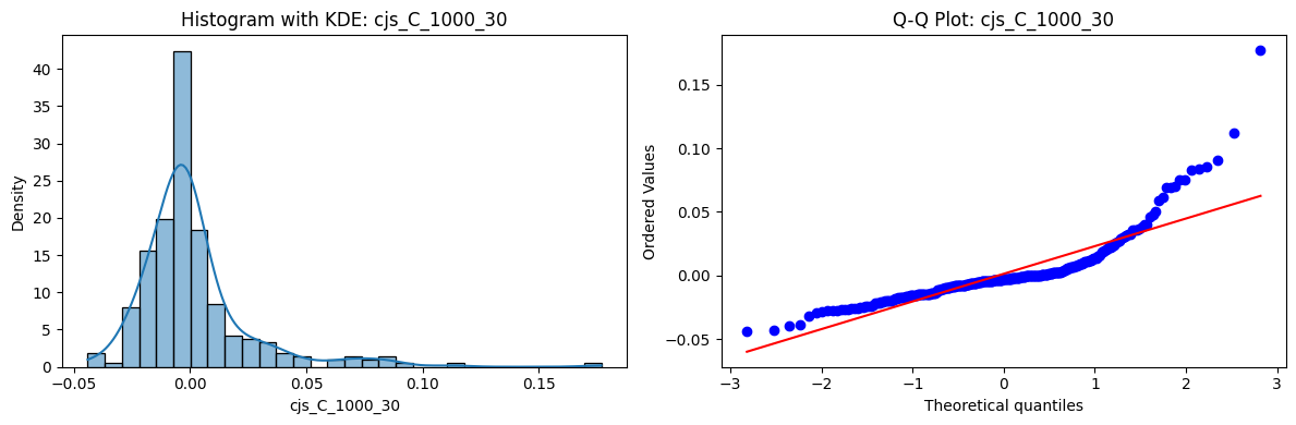
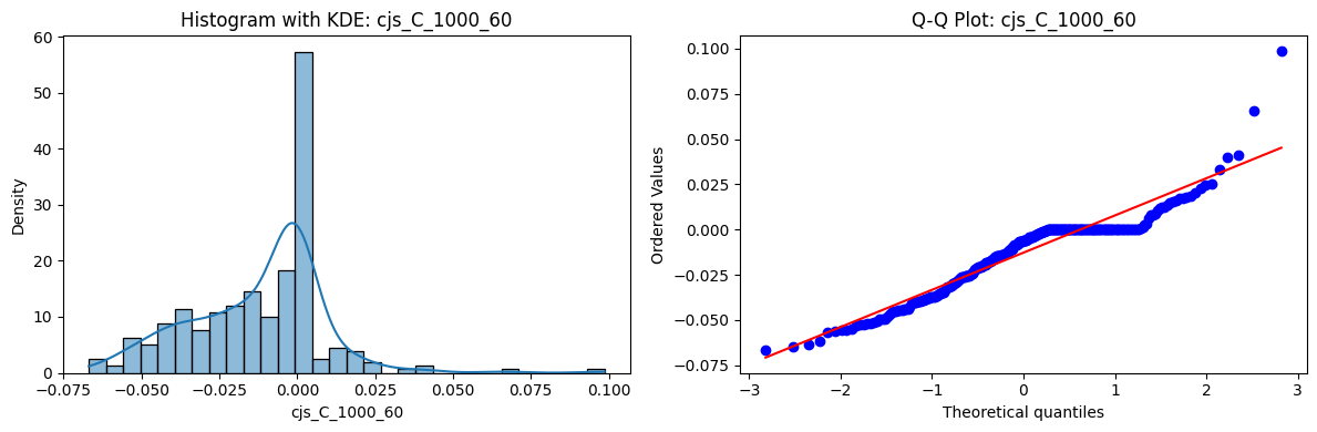
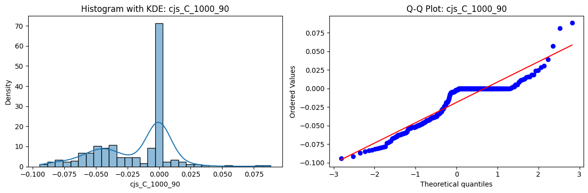
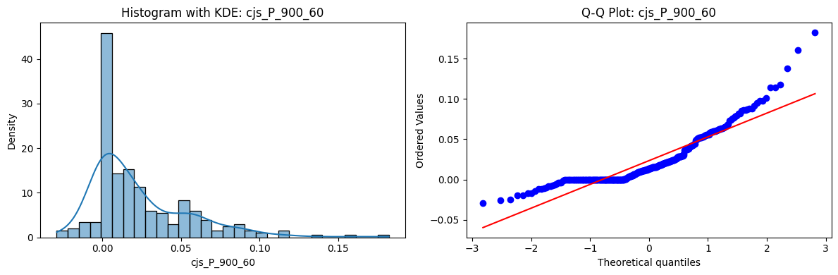
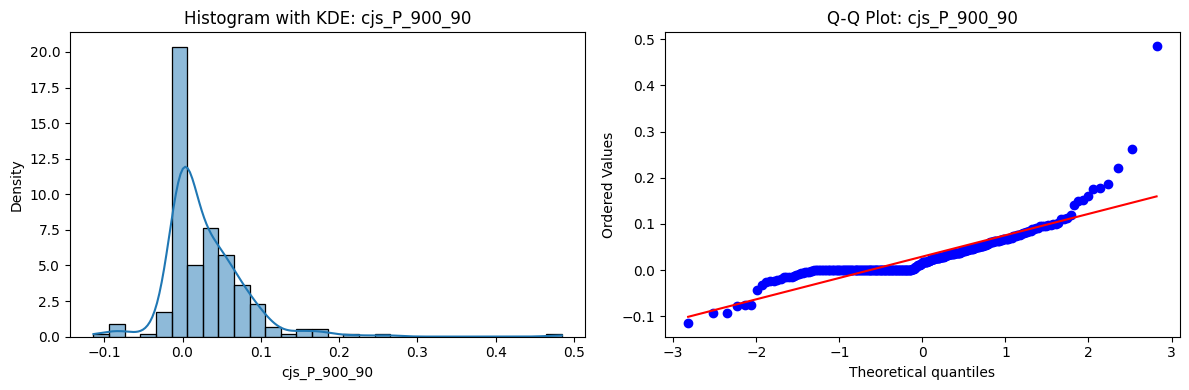
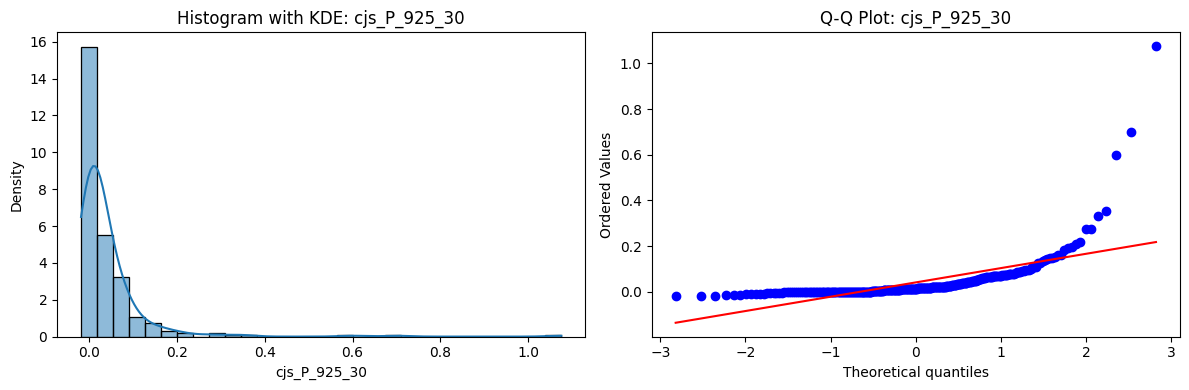
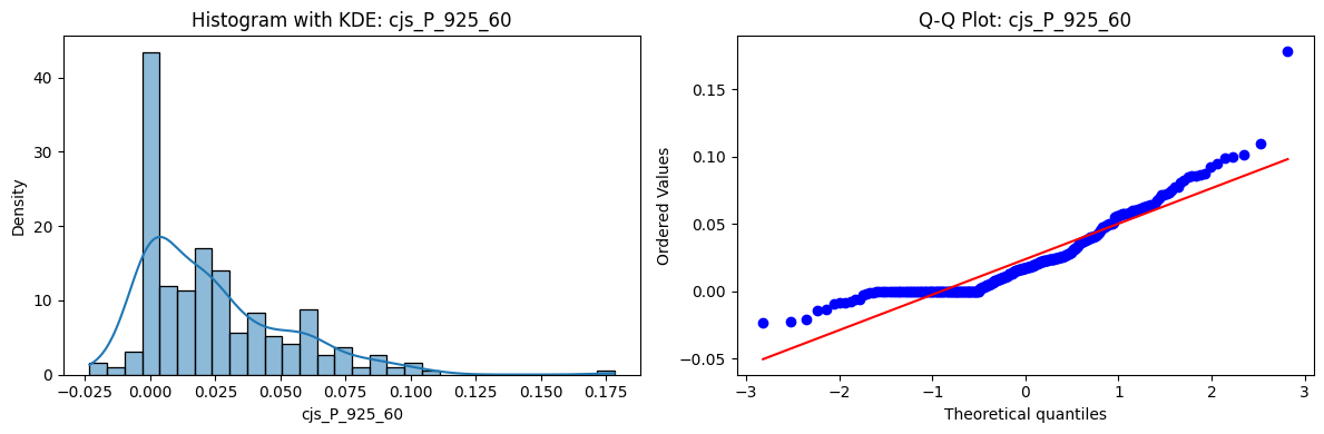
Tests for Normality of Returns in the 54 CJS Portfolios

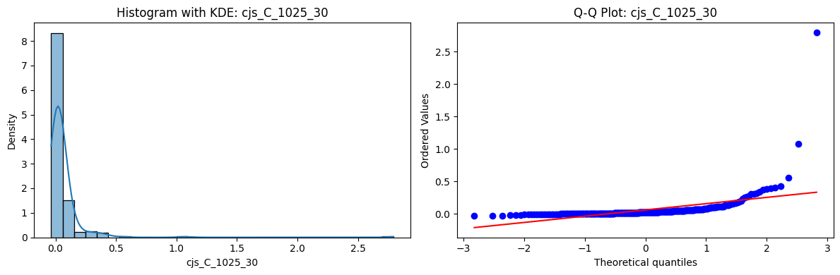
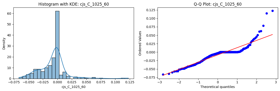
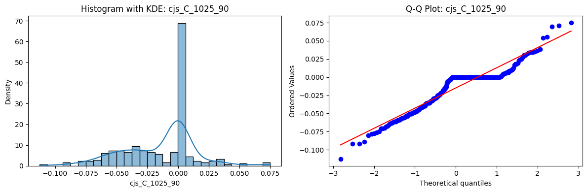
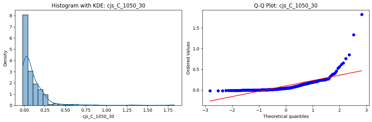
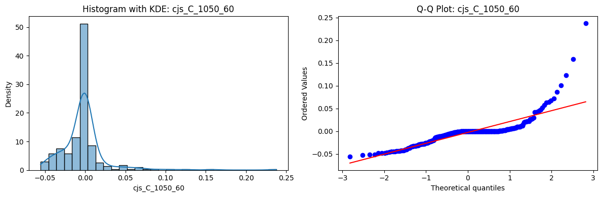
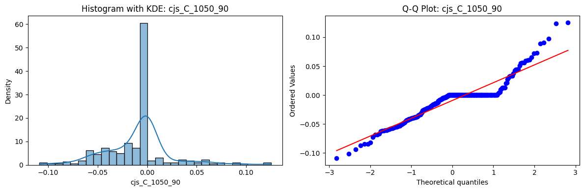
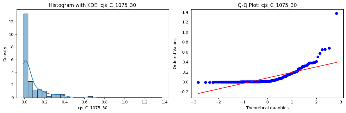
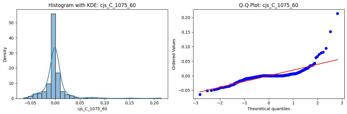
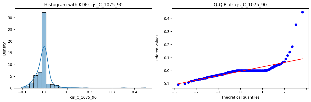
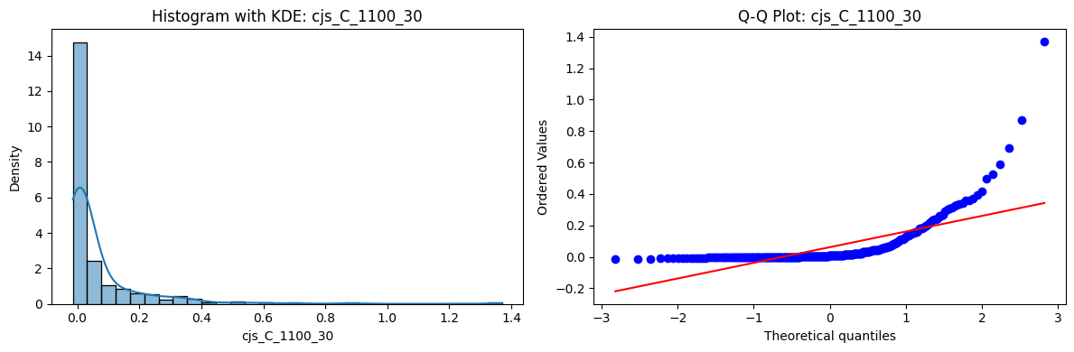
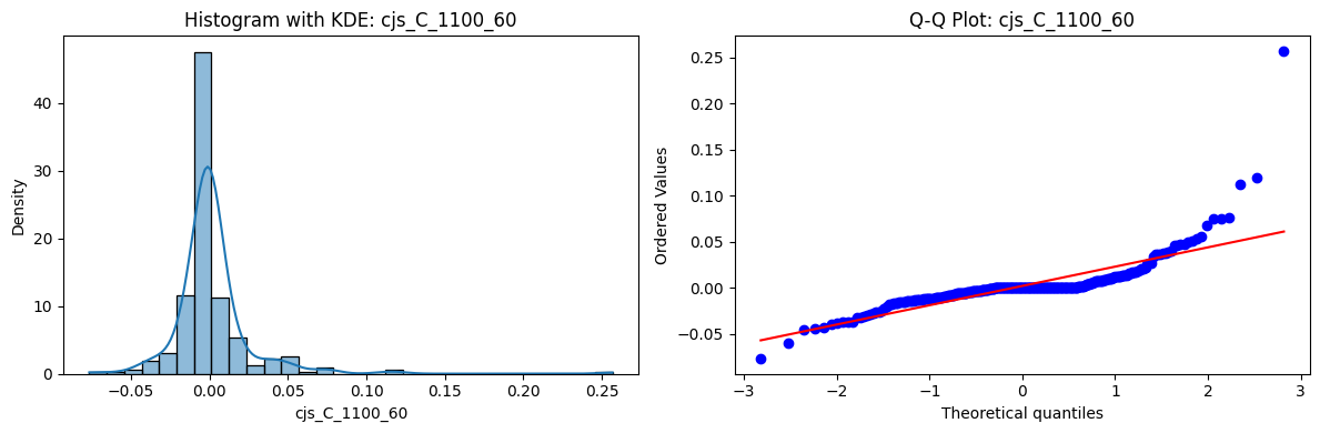
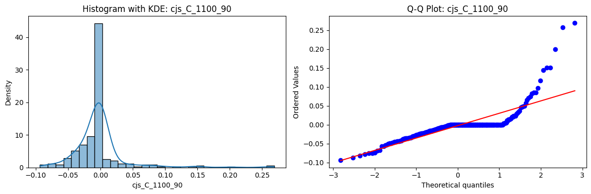
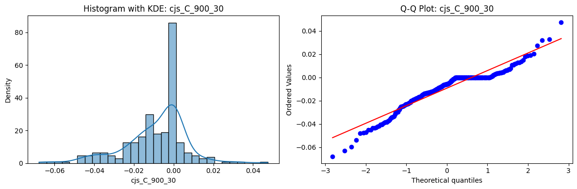
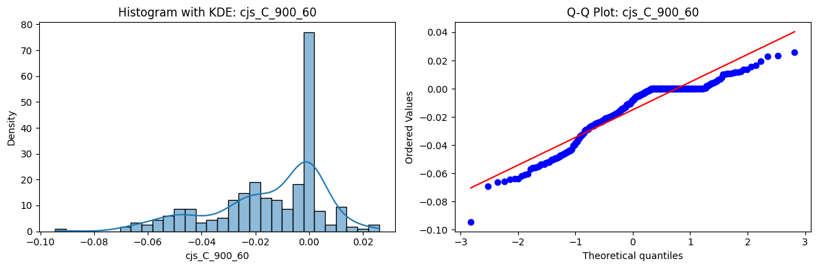
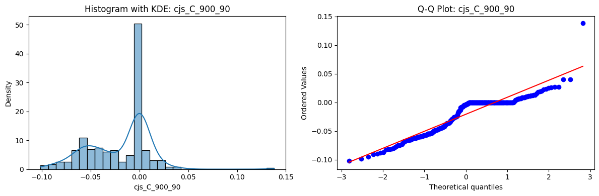
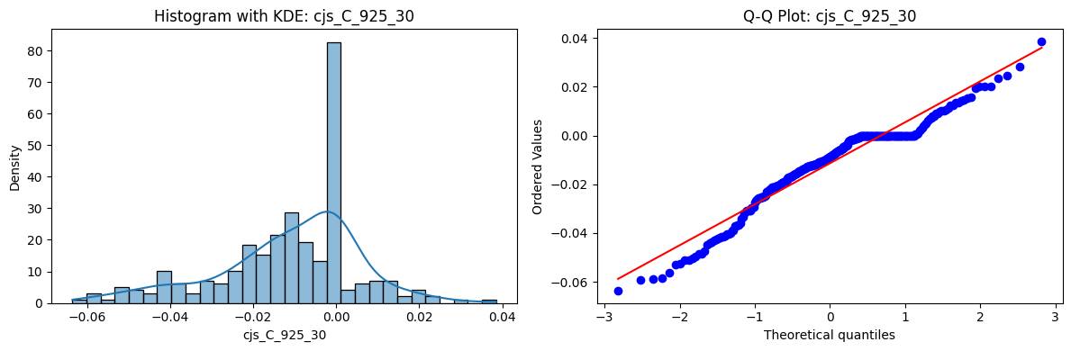
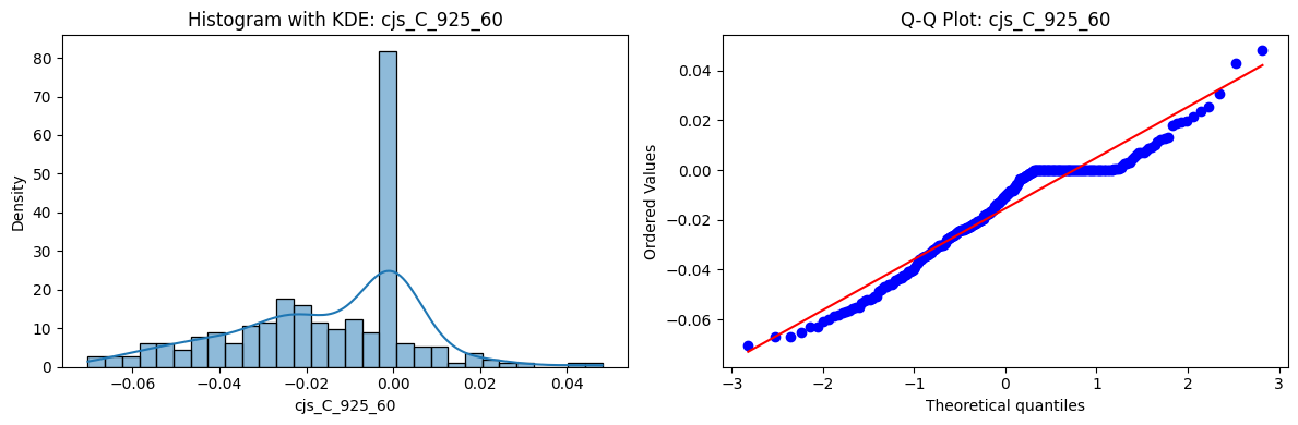
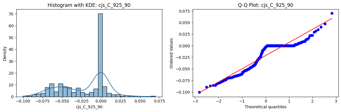
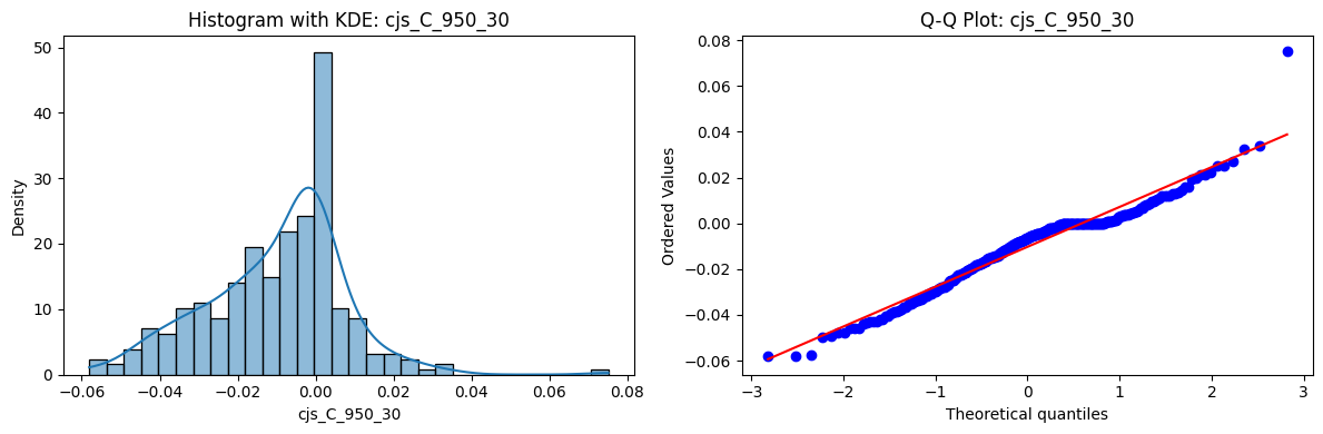
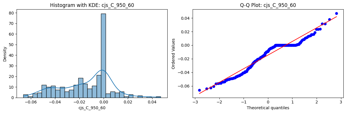
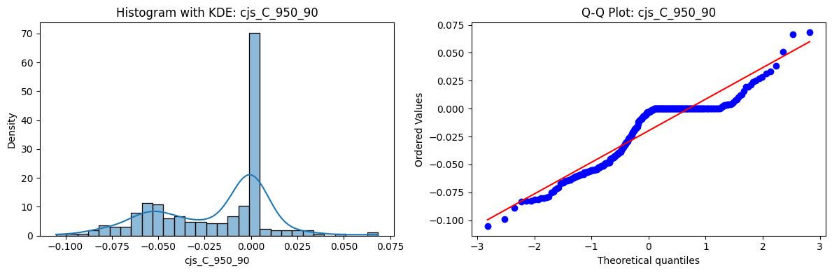
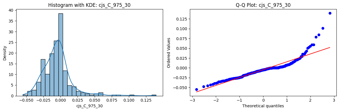
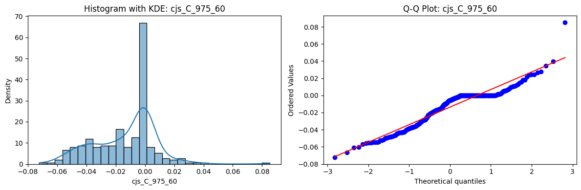
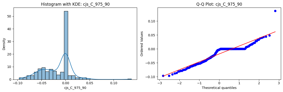
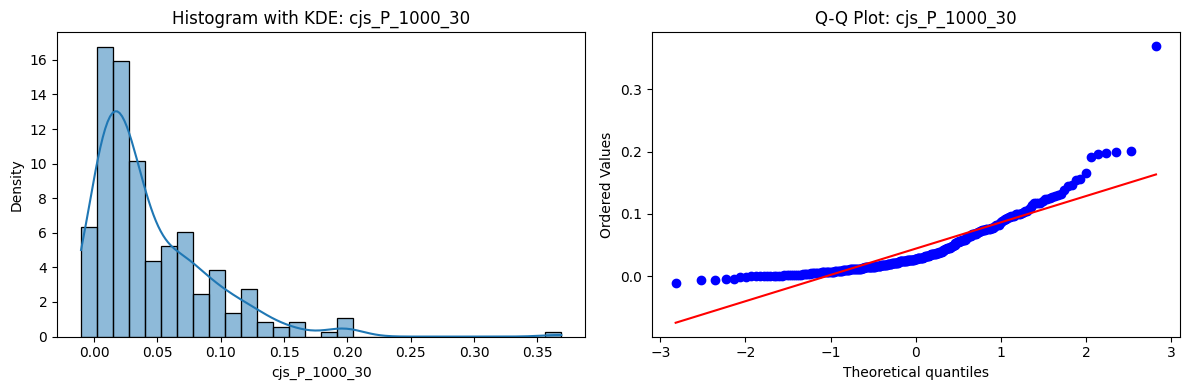
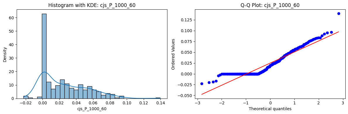
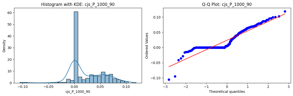
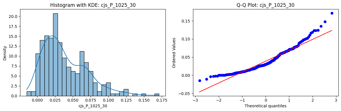
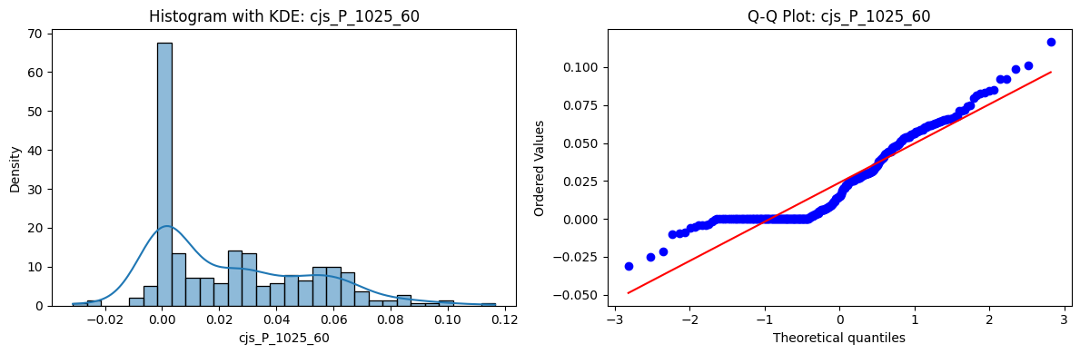
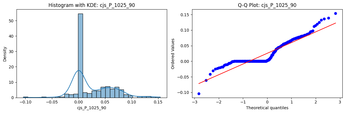
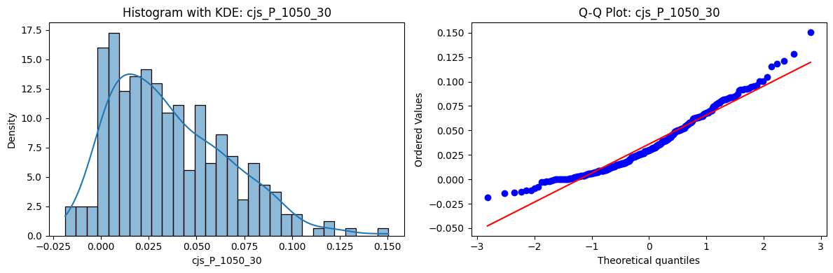
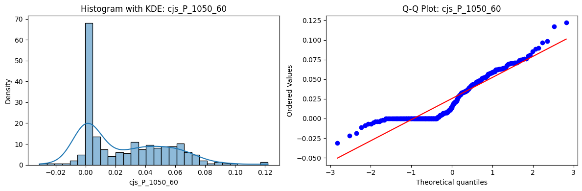
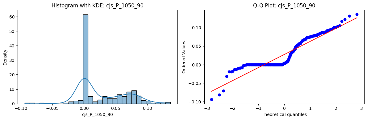
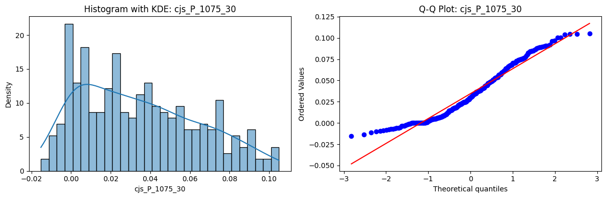
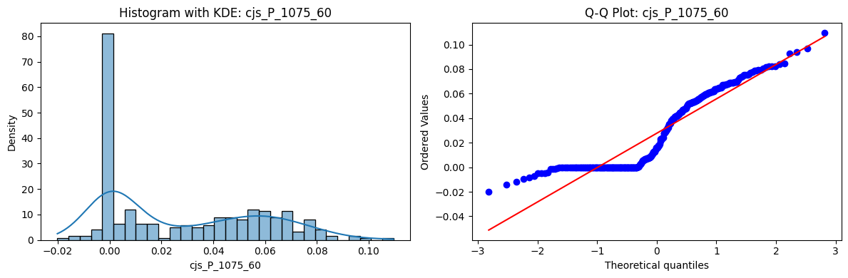
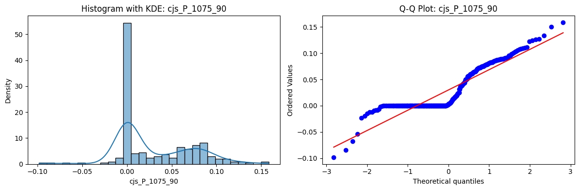
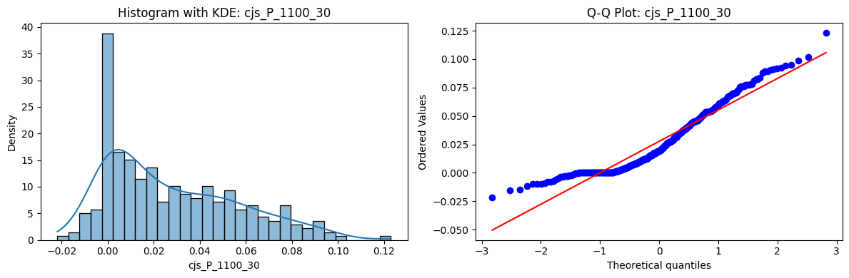
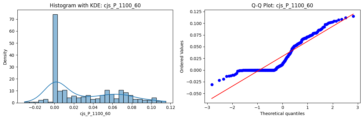
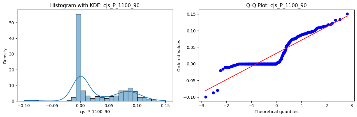
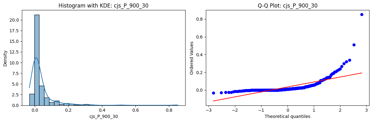
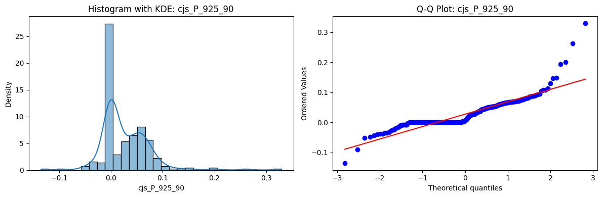
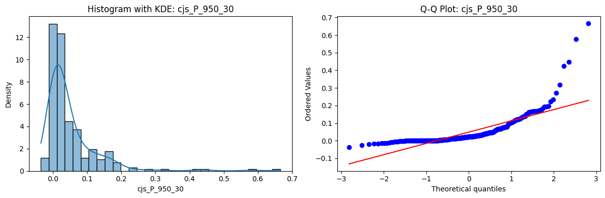
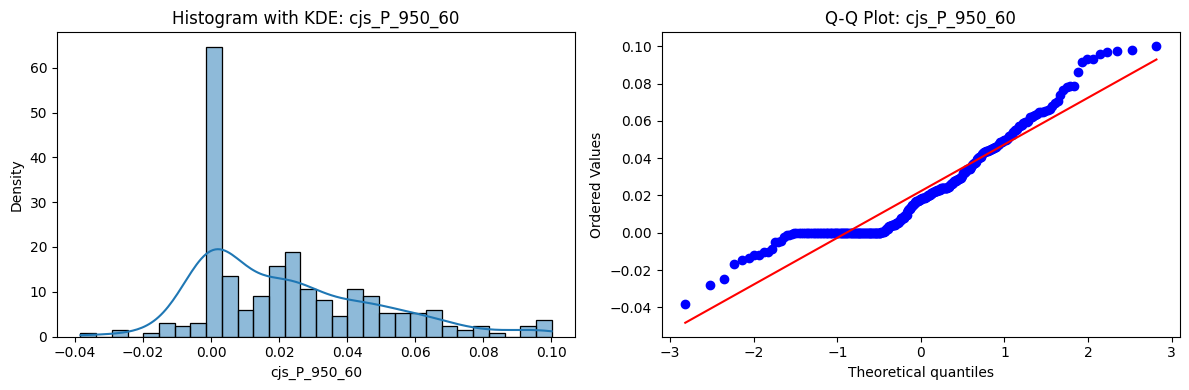
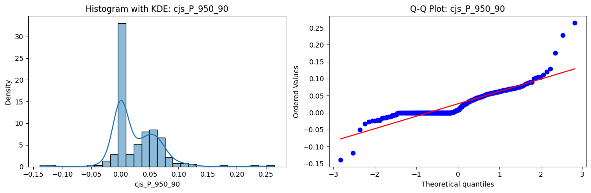
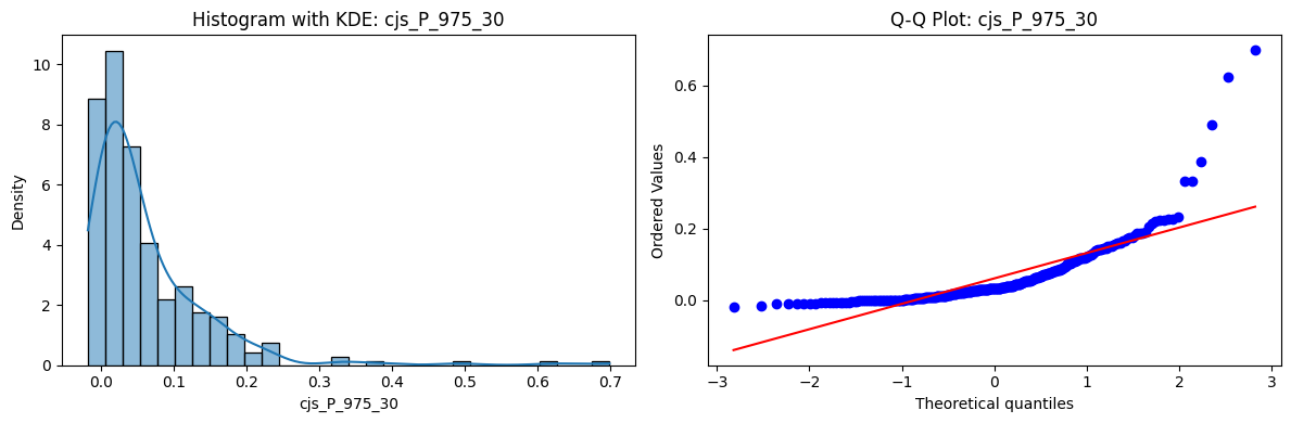
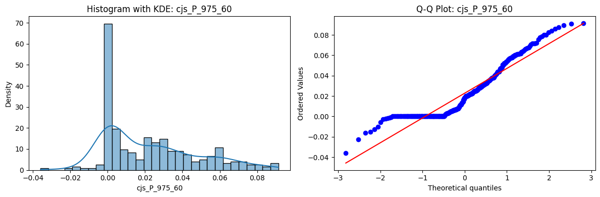
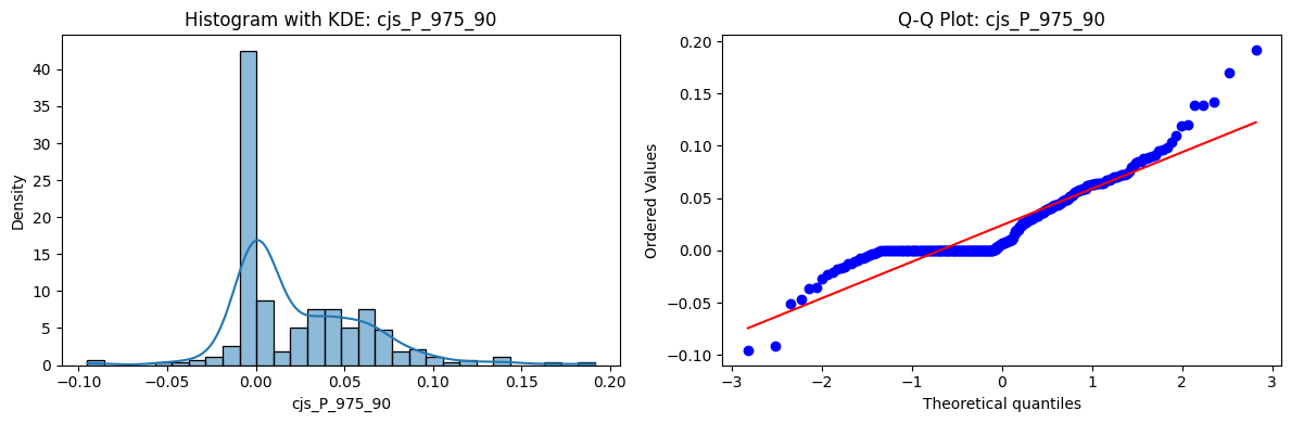
Distributions and Q-Q plots of the 54 CJS portfolios are shown below, based on the filtration and portfolio construction we have implemented.

Normality Tests (Shapiro, Jarque-Bera, Normaltest p-values): All means and medians ≈ 0, with maximums < 0.05. This indicates systematic rejection of normality at conventional significance levels (1% and 5%) for essentially all portfolios. In other words: none of these return distributions look Gaussian.

Skewness: Mean skewness ≈ 1.64, median ≈ 0.77 → distributions tend to be right-skewed (long right tails). Wide spread (std ≈ 2.26; max ≈ 11.1, min ≈ -0.91) → some portfolios are extremely positively skewed, while a few have mild negative skew.

Kurtosis: Mean kurtosis ≈ 14.5, median ≈ 4.6 (close to normal’s 3, but slightly higher). Very large spread (std ≈ 23.8; max ≈ 152.7) → many distributions are leptokurtic (fat-tailed). Averages are pulled up by extreme outliers, meaning some portfolios experience rare but massive return shocks.

returns_df = cjs_returns.copy()
returns_df = returns_df.reset_index().pivot_table(
    columns="ftfsa_id", index="date", values="return"
)

# Apply to returns dataframe
summary_df = normality_summary(returns_df)
display(summary_df.describe().style.format(na_rep="NaN", precision=5, thousands=","))

# Plot histogram and QQ plot for each series
for col in returns_df.columns:
    fig, axs = plt.subplots(1, 2, figsize=(12, 4))

    sns.histplot(returns_df[col].dropna(), kde=True, stat="density", bins=30, ax=axs[0])
    axs[0].set_title(f"Histogram with KDE: {col}")

    stats.probplot(returns_df[col].dropna(), dist="norm", plot=axs[1])
    axs[1].set_title(f"Q-Q Plot: {col}")

    plt.tight_layout()
    plt.show()

	Shapiro_p	JarqueBera_p	Normaltest_p	Skewness	Kurtosis
count	54.00000	54.00000	54.00000	54.00000	54.00000
mean	0.00000	0.00228	0.00276	1.63759	14.52659
std	0.00000	0.00805	0.00801	2.25902	23.79816
min	0.00000	0.00000	0.00000	-0.90799	1.83906
25%	0.00000	0.00000	0.00000	0.22364	2.98662
50%	0.00000	0.00000	0.00000	0.77120	4.61425
75%	0.00000	0.00000	0.00003	2.87608	18.37195
max	0.00000	0.04874	0.04428	11.10561	152.67355

---

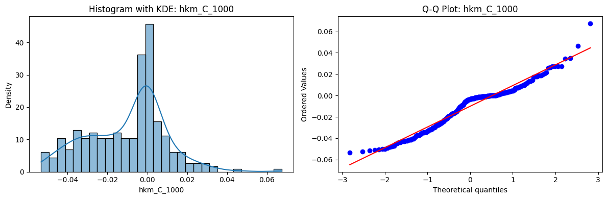
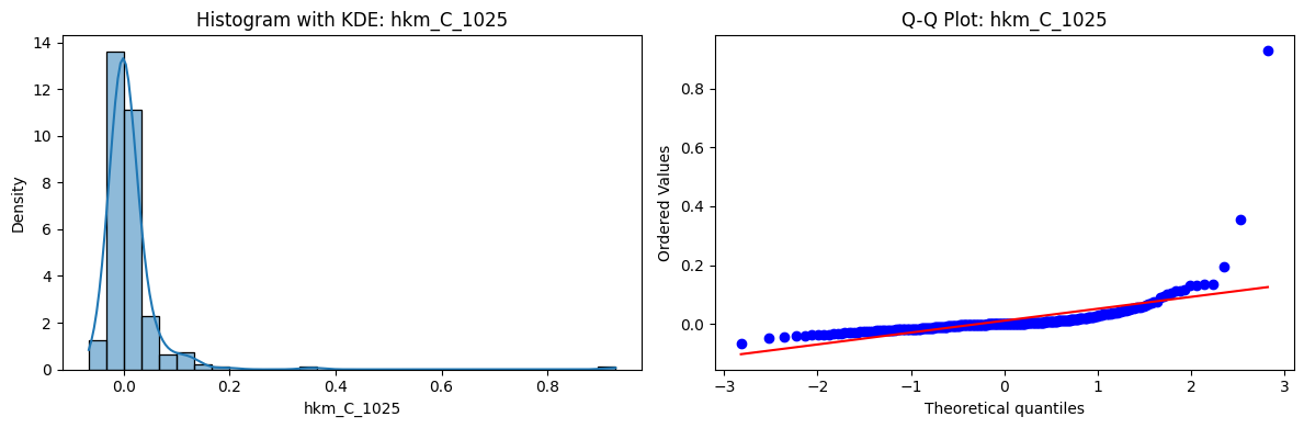
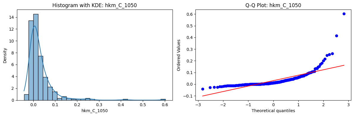
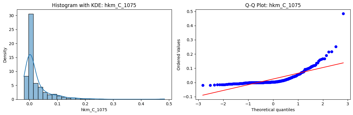
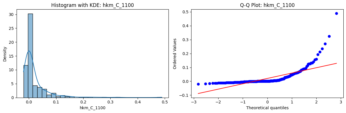
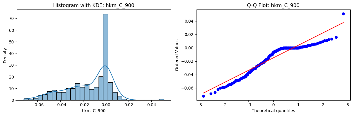
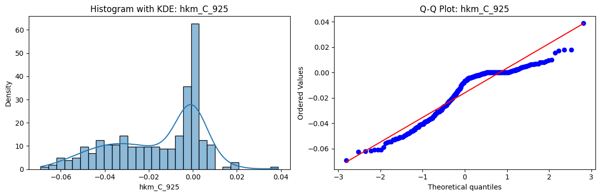
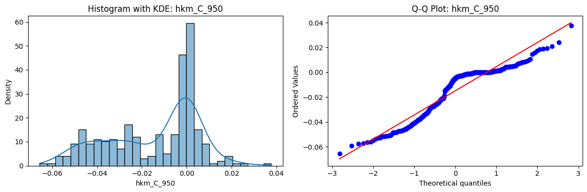
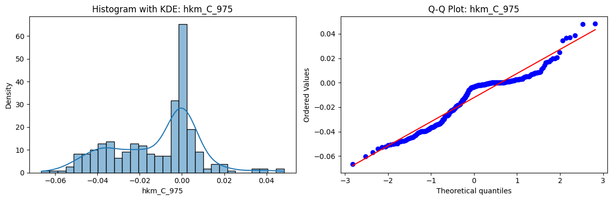
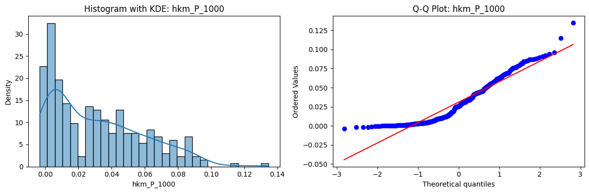
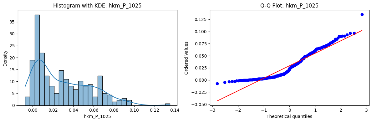
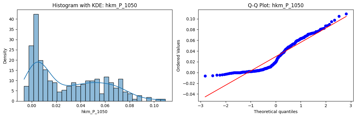
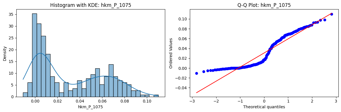
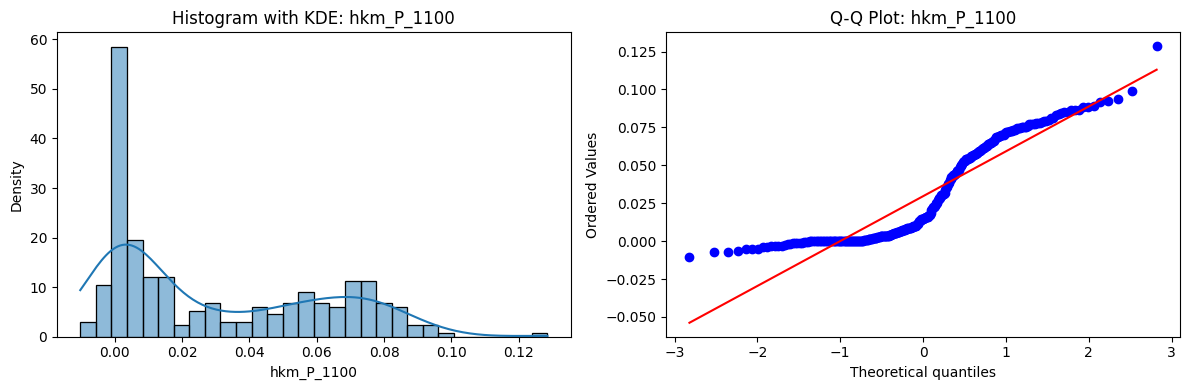
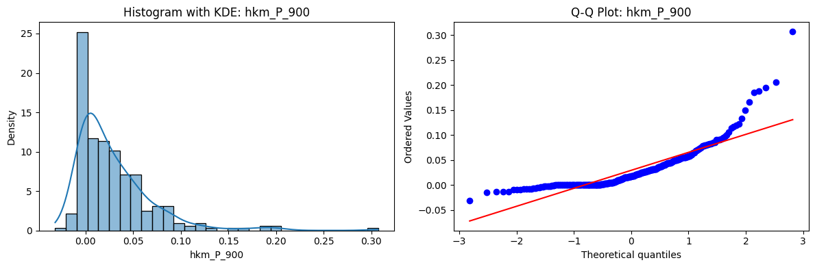
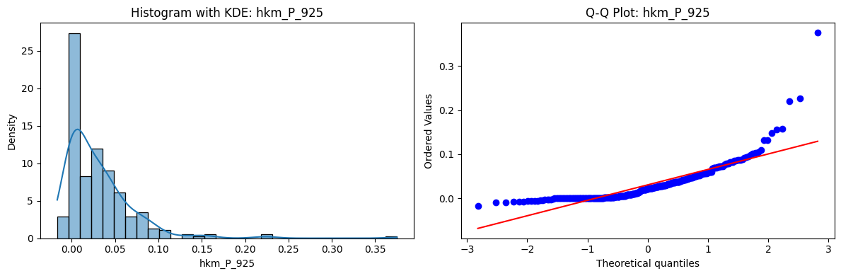
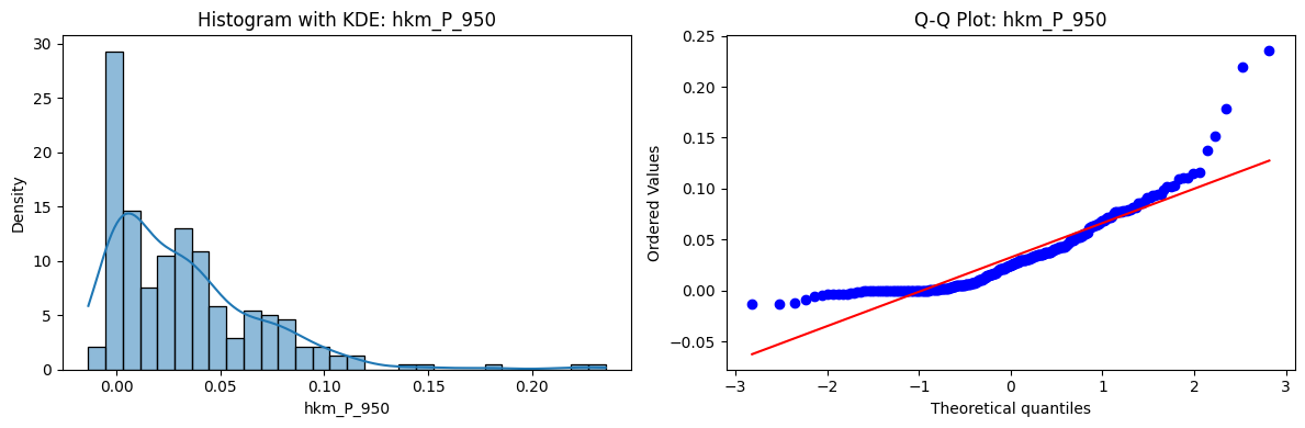
Tests for Normality of Returns in the 18 HKM Portfolios

Distributions and Q-Q plots of the 18 HKM portfolios are shown below, based on the filtration and portfolio construction we have implemented.

Normality Tests:

• Shapiro p-values: all 0 → normality always rejected.

• Jarque-Bera & Normaltest p-values: means ~0.05, with maximums up to ~0.70 and ~0.61 respectively. Some portfolios do not reject normality at the 5% level, unlike the first dataset (where rejection was universal). Suggests a few return distributions here are closer to Gaussian, but the majority still deviate.

Skewness: Mean ≈ 1.87, median ≈ 0.78, similar to the first set (mean ≈ 1.64). Distribution wider: standard deviation ≈ 2.64, maximum ≈ 9.8. Takeaway: again, portfolios are generally positively skewed, with several highly right-tailed portfolios.

Kurtosis: Mean ≈ 16.8, median ≈ 3.1. This median is much closer to normal (3.0) than in the first dataset (median ≈ 4.6). Spread large (std ≈ 30.3, max ≈ 129.3) → still evidence of extreme fat tails in some cases, but fewer portfolios appear strongly leptokurtic compared to the first set. Comparison with the 54-Portfolios Set

returns_df = hkm_returns.copy()
returns_df = returns_df.reset_index().pivot_table(
    columns="ftfsa_id", index="date", values="return"
)

# Apply to returns dataframe
summary_df = normality_summary(returns_df)
display(summary_df.describe().style.format(na_rep="NaN", precision=5, thousands=","))

# Plot histogram and QQ plot for each series
for col in returns_df.columns:
    fig, axs = plt.subplots(1, 2, figsize=(12, 4))

    sns.histplot(returns_df[col].dropna(), kde=True, stat="density", bins=30, ax=axs[0])
    axs[0].set_title(f"Histogram with KDE: {col}")

    stats.probplot(returns_df[col].dropna(), dist="norm", plot=axs[1])
    axs[1].set_title(f"Q-Q Plot: {col}")

    plt.tight_layout()
    plt.show()

	Shapiro_p	JarqueBera_p	Normaltest_p	Skewness	Kurtosis
count	18.00000	18.00000	18.00000	18.00000	18.00000
mean	0.00000	0.05090	0.04631	1.86917	16.77614
std	0.00000	0.16958	0.15018	2.64475	30.26227
min	0.00000	0.00000	0.00000	-0.70095	1.84262
25%	0.00000	0.00000	0.00000	0.08527	2.46929
50%	0.00000	0.00000	0.00000	0.77842	3.09835
75%	0.00000	0.00001	0.00000	3.12405	20.20166
max	0.00000	0.69876	0.60995	9.83980	129.33881