Homework 2: Numpy, Scipy, and Matplotlib#

Intructions

In this problem set, we’ll be learning the basics of Numpy, Scipy, and Matplotlib.

A blank code or markup cell will be left after each exercise for you to fill in with your solution.

I’ve completed the first few exercises for you to show you how you should format your HW submission.

Import Necessary Modules#

You should always start you file with all of the import statements that you will be using for the file. This makes it easier to quickly check what modules each file depends on—all you have to do is look at the top of the file.

For this problem, import numpy, scipy, and the pyplot submodule from matplotlib.

# Completed for you

import numpy as np
import pandas as pd
import scipy
import scipy.integrate
import scipy.stats
from scipy import misc
from scipy.optimize import minimize
from matplotlib import pyplot as plt

Q1. Use built-in Numpy functions to do the following tasks#

Create a vector (numpy array) of size 10 that contains all zeros and print it. (Use np.zeros.)
Use arange to create a vector of values from 5 to 24. Print it.
Use arange and Python “slicing” to create a vector of values from 24, to 5. Print it.
Use arange and Python “slicing” to create a vector consisting of all the even integers in the half-open interval $[0,30)$.
Use arange and reshape to create a 3x3 numpy array containing the numbers 0 to 8.

# Completed for you

# 1
print("1.")
Z = np.zeros(10)
print(Z)

# 2
print("2.")
print(np.arange(5,25))

# 3
print("3.")
z = np.arange(5, 25)
print(z[::-1])

# 4
print("4.")
z = np.arange(0,30)
print(z[::2])

# 5
print("5.")
print(np.arange(0,9).reshape((3,3)))

1.
[0. 0. 0. 0. 0. 0. 0. 0. 0. 0.]
2.
[ 5  6  7  8  9 10 11 12 13 14 15 16 17 18 19 20 21 22 23 24]
3.
[24 23 22 21 20 19 18 17 16 15 14 13 12 11 10  9  8  7  6  5]
4.
[ 0  2  4  6  8 10 12 14 16 18 20 22 24 26 28]
5.
[[0 1 2]
 [3 4 5]
 [6 7 8]]

Q2. Numpy functions continued… (2 points each)#

Use eye to create a 5x5 identity matrix. Print it.
Use random.random to generate a 3x3x3 array of numbers randomly generated from a uniform distribution over the support interval $[0,1)$. Print it.
Create a 10x10 array with similarly generated random values. Find and print the minimum and maximum values appearing in the matrix using min and max.
Create a random vector of size 30. Find and print the mean value.
Use zeros and/or ones and slicing to create a 10x10 array with 1’s on the border and 0’s inside.

# TODO
print("1.")
print("2.")
print("3.")
print("4.")
print("5.")

1.
2.
3.
4.
5.

Q3. Integration with Scipy (2 points)#

(1) The PDF of a Normal distibution is $$ f(x; \mu, \sigma) = \frac{1}{\sqrt{2 \pi \sigma^2}} \exp\left\{- \frac{(x - \mu)^2}{2 \sigma^2}\right\} $$

Let $\mu = 1$ and $\sigma = 2$. Use Scipy to numerical integrate this function. Specifically, calculate $$ \int_{-2}^{2} f(x; \mu, \sigma) \mathrm d x $$

Verify your result using the built-in function for the CDF of a normal distribution: scipy.stats.norm.cdf(x, loc=mu, scale=sigma). To calculate the proper area as the integral above, you will need to compute $$ F(2) - F(-2), $$ where $F$ is the CDF of the normal with mean 1 and standard deviation 2.

(Hint: You will need to import scipy.integrate and scipy.stats to access the functions that you need.)

# TODO

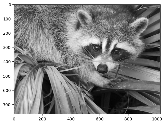
Q4. Array Indexing with an Image (4 points)#

Run the code in the cell below to access a matrix called face. Print the matrix to get an idea of what it looks like. What is its dimensions?

from scipy import misc
face = misc.face(gray=True).astype('float64')

/var/folders/l3/tj6vb0ld2ys1h939jz0qrfrh0000gn/T/ipykernel_13107/127514662.py:2: DeprecationWarning: scipy.misc.face has been deprecated in SciPy v1.10.0; and will be completely removed in SciPy v1.12.0. Dataset methods have moved into the scipy.datasets module. Use scipy.datasets.face instead.
  face = misc.face(gray=True).astype('float64')

# TODO

Use the following code to plot the elements of the matrix as an image: plt.imshow(face, cmap=plt.cm.gray)

# TODO

Now, apply the function np.sin(x/25) to the face matrix and then plot it again. This doesn’t do anything very deep, it just messes with the shades of gray in a nonlinear way.

Note: Do not permanently alter the face matrix with this transformation. If you wish, you may create a new matrix called face_sine, but you don’t need to. We won’t be using this transformed matrix after this step. This was just for practice.

# TODO

Imagine a circle with a center at the matrix indices (300, 620) and a radius of 250. In the x-y plane, this would be 620, 300. Write a snippet of code that, for each pixel, calculates the distance of that pixel from the center of this circle. If the distance is greater than the radius of the circle, set the value of the pixel (the element of the matrix) equal to zero. Plot the result, again using plt.ishow with a gray colormap.

Be sure to create a new copy of the face matrix, face2. Create a proper copy using the copy method of the np.array class.

# TODO: Finish the following code.

face2 = face.copy()
cx, cy = 620, 300
radius = 250
for i in range(face.shape[0]):
    for j in range(face.shape[1]):        
        # TODO: Your code here
        pass
        
plt.imshow(face2, cmap=plt.cm.gray)

<matplotlib.image.AxesImage at 0x16d3df950>

../_images/a1891888c12252f4686dc4ce3d66a90a24cef63c5c8e27251870a6e11a40784d.png

Q5. Fitting a Curve to Data (2 points for each part)#

In this exercise, you will fit a nonlinear curve to data by minimizing the sum of squares. Below, I have given data and a function to plot the data and a curve over the data. The curve is the following function: $$ y(t) = x_0 \exp(-x_2 t) + x_1 \exp(-x_3 t). $$

from scipy.optimize import minimize
data = np.array(
  [[0.0000, 5.8955], 
   [0.1000, 3.5639],
   [0.2000, 2.5173],
   [0.3000, 1.9790],
   [0.4000, 1.8990],
   [0.5000, 1.3938],
   [0.6000, 1.1359],
   [0.7000, 1.0096],
   [0.8000, 1.0343],
   [0.9000, 0.8435],
   [1.0000, 0.6856],
   [1.1000, 0.6100],
   [1.2000, 0.5392],
   [1.3000, 0.3946],
   [1.4000, 0.3903],
   [1.5000, 0.5474],
   [1.6000, 0.3459],
   [1.7000, 0.1370],
   [1.8000, 0.2211],
   [1.9000, 0.1704],
   [2.0000, 0.2636]])

def plot_against_data(x):
    tgrid = data[:,0]
    ydata = data[:,1]
    yfunc = lambda t: x[0] * np.exp(-x[2]* t) + x[1] * np.exp(-x[3] * t)
    y = yfunc(tgrid)
    plt.plot(tgrid, ydata, '.')
    plt.plot(tgrid, y)
    
x_initial = np.array([1, 1, 1, 0])

(1): Use the given plotting function to plot the data and the curve for the given initial guess of the parameters, x_initial.

# TODO

(2) Write a function called sum_squares that takes in a vector of model paraters (e.g., x_initial) and returns the sum of squares that results from the difference of the data and the curve defined by x_initial. What is the sum of squares that results from the given x_initial?

# TODO

(3) Use scipy.optimize.minimize to minimize the sum of squares, using the function that you wrote previously. Save the optimal parameters to the variable xstar.

# TODO

(4) Use the plot_against_data function that was given to plot the optimal curve, defined by xstar, against the data.

# TODO

Q6. Compressing an Image with Linear Algebra (2 points for each part)#

Here we’ll play with the Singular Value Decomposition (SVD) function in Numpy’s linalg submodule. You can think of the SVD as a generalization of the eigenvalue decomposition for non-square matrices.

Here we will be using the same face matrix as above.

(1) To begin, calculate the SVD using the code. (For this part, you can just copy and paste this code.)

u, s, v = np.linalg.svd(face, full_matrices=False)

# TODO

(2) Calculate the shape of u, s, and v.

# TODO

(3) Construct a matrix by matrix multiplying u, s, and v. Note that s doesn’t conform as it stands. Mathematically, we want to compute $$ U \cdot \text{diag}(S) \cdot V. $$ Thus, we need $\text{diag}(S)$ to be a 768 x 768 matrix with the values of s on the diagonal. These are the singular values—analogous to the eigenvalues—of the face matrix. Use np.diag to do this. Use @ to perform the matrix multplication. Call this new matrix faceUSV.

# TODO

(4) Use the function np.allclose to test if all of the elements of the matrices faceUSV and face are numerically close. Does this verify that our reconstruction was successful? Why are we using np.allclose instead of, say, faceUSV == face to test if the matrices are the same?

# TODO

(5) Now, construct a function called compress that takes in a number n and returns a matrix constructed as follows:

\[ U_n \cdot \text{diag}(S_n) \cdot V_n \]

where $U_n$ is only the first n columns of the matrix u, $\text{diag}(S_n)$ is the first n singular values put on the diagonals of a matrix of zeros (hint: np.diag(s[0:n])), and $V_n$ is the first n rows of the matrix v.

# TODO

(6) Use your newly created compress function to create the a matrix called face_compressed for various values of n. Plot the matrix using plt.imshow(face_compressed, cmap=plt.cm.gray). Do this for n in [500, 300, 100, 50, 10]. What do you see happening?

# TODO

(7). Again use the size method to calculate the number of “pixels” (elements in the array) that are in the original face matrix. Now, suppose we use the SVD to store this image. Write a function called storage_size that computes that number of elements in $U_r$, the number of elements in $V_r$, adds them together, and then adds $n$ for the number of singular values of the $S_r$ vector used. That is

\[ storageSize = numberOfElements(U_n) + numberOfElements(V_n) + numberOfElements(S_n) \]

# TODO

(8) Compute the storage size for each of the values of n that we tested above. Compared to the original size, face.size, how much space are we saving (in percentages) when we use n=100 (which looks almost lossless)?

# TODO

NOTE: Essentially, we are reconstructing the matrix (and image) using the first n singular values. Equivalently, we could say that we are using Principal Component Analysis and reconstructing the image using the first n principal components. If this were a square matrix, we could say that we are using the first n eigenvalues and eigenvectors.

We will later see that this same technique can be used to analyze complex data. Imagine, for example, applying this procedure to a matrix of data or to the variance-covariance matrix of a set of variables. We will later see that, in the same way that we are compressing and summarizing a complex image, we can summarize the joint distribution of a set of variables.

Homework 2: Numpy, Scipy, and Matplotlib

Contents