4.5 Factor Analysis on Financial and Economic Time Series

Factor Analysis and Principal Component Analysis on Financial and Economic Time Series

# If you're running this on Colab, make sure to install the following packages using pip.
# On you're own computer, I recommend using conda or mamba.

# !pip install pandas-datareader
# !pip install yfinance

# !conda install pandas-datareader
# !conda install yfinance

import numpy as np
import pandas as pd
from matplotlib import pyplot as plt

import yfinance as yf
import pandas_datareader as pdr
import sklearn.decomposition
import statsmodels.multivariate.pca

import config
DATA_DIR = config.DATA_DIR

Downloading macroeconomic and financial data from FRED

fred_series_long_names = {
    'BAMLH0A0HYM2': 'ICE BofA US High Yield Index Option-Adjusted Spread',
    'NASDAQCOM': 'NASDAQ Composite Index',
    'RIFSPPFAAD90NB': '90-Day AA Financial Commercial Paper Interest Rate',
    'TB3MS': '3-Month Treasury Bill Secondary Market Rate',
    'DGS10': 'Market Yield on U.S. Treasury Securities at 10-Year Constant Maturity',
    'VIXCLS': 'CBOE Volatility Index: VIX',
}

fred_series_short_names = {
    'BAMLH0A0HYM2': 'High Yield Index OAS',
    'NASDAQCOM': 'NASDAQ',
    'RIFSPPFAAD90NB': '90-Day AA Fin CP',
    'TB3MS': '3-Month T-Bill',
    'DGS10': '10-Year Treasury',
    'VIXCLS': 'VIX',
}

start_date = pd.to_datetime('1980-01-01') 
end_date = pd.to_datetime('today') 

df = pdr.get_data_fred(fred_series_short_names.keys(), start=start_date, end=end_date)

First, an aside about reading and writing data to disk.

df.to_csv(DATA_DIR / 'fred_panel.csv')

dff = pd.read_csv(DATA_DIR / 'fred_panel.csv')

dff.info()

<class 'pandas.core.frame.DataFrame'>
RangeIndex: 12155 entries, 0 to 12154
Data columns (total 7 columns):
 #   Column          Non-Null Count  Dtype  
---  ------          --------------  -----  
 0   DATE            12155 non-null  object 
 1   BAMLH0A0HYM2    7472 non-null   float64
 2   NASDAQCOM       11500 non-null  float64
 3   RIFSPPFAAD90NB  6606 non-null   float64
 4   TB3MS           547 non-null    float64
 5   DGS10           11405 non-null  float64
 6   VIXCLS          8994 non-null   float64
dtypes: float64(6), object(1)
memory usage: 664.9+ KB

dff = pd.read_csv(DATA_DIR / 'fred_panel.csv', parse_dates=['DATE'])

dff.info()

<class 'pandas.core.frame.DataFrame'>
RangeIndex: 12155 entries, 0 to 12154
Data columns (total 7 columns):
 #   Column          Non-Null Count  Dtype         
---  ------          --------------  -----         
 0   DATE            12155 non-null  datetime64[ns]
 1   BAMLH0A0HYM2    7472 non-null   float64       
 2   NASDAQCOM       11500 non-null  float64       
 3   RIFSPPFAAD90NB  6606 non-null   float64       
 4   TB3MS           547 non-null    float64       
 5   DGS10           11405 non-null  float64       
 6   VIXCLS          8994 non-null   float64       
dtypes: datetime64[ns](1), float64(6)
memory usage: 664.9 KB

dff = dff.set_index('DATE')

df.to_parquet(DATA_DIR / 'fred_panel.parquet')

df = pd.read_parquet(DATA_DIR / 'fred_panel.parquet')

df.info()

<class 'pandas.core.frame.DataFrame'>
DatetimeIndex: 12155 entries, 1980-01-01 to 2025-08-14
Data columns (total 6 columns):
 #   Column          Non-Null Count  Dtype  
---  ------          --------------  -----  
 0   BAMLH0A0HYM2    7472 non-null   float64
 1   NASDAQCOM       11500 non-null  float64
 2   RIFSPPFAAD90NB  6606 non-null   float64
 3   TB3MS           547 non-null    float64
 4   DGS10           11405 non-null  float64
 5   VIXCLS          8994 non-null   float64
dtypes: float64(6)
memory usage: 664.7 KB

df

	BAMLH0A0HYM2	NASDAQCOM	RIFSPPFAAD90NB	TB3MS	DGS10	VIXCLS
DATE
1980-01-01	NaN	NaN	NaN	12.0	NaN	NaN
1980-01-02	NaN	148.17	NaN	NaN	10.50	NaN
1980-01-03	NaN	145.97	NaN	NaN	10.60	NaN
1980-01-04	NaN	148.02	NaN	NaN	10.66	NaN
1980-01-07	NaN	148.62	NaN	NaN	10.63	NaN
...	...	...	...	...	...	...
2025-08-08	2.94	21450.02	4.21	NaN	4.27	15.15
2025-08-11	2.94	21385.40	4.23	NaN	4.27	16.25
2025-08-12	2.93	21681.90	4.20	NaN	4.29	14.73
2025-08-13	2.90	21713.14	4.18	NaN	4.24	14.49
2025-08-14	2.89	21710.67	4.22	NaN	NaN	14.83

12155 rows × 6 columns

Cleaning Data

df = dff.rename(columns=fred_series_short_names)
df

	High Yield Index OAS	NASDAQ	90-Day AA Fin CP	3-Month T-Bill	10-Year Treasury	VIX
DATE
1980-01-01	NaN	NaN	NaN	12.0	NaN	NaN
1980-01-02	NaN	148.17	NaN	NaN	10.50	NaN
1980-01-03	NaN	145.97	NaN	NaN	10.60	NaN
1980-01-04	NaN	148.02	NaN	NaN	10.66	NaN
1980-01-07	NaN	148.62	NaN	NaN	10.63	NaN
...	...	...	...	...	...	...
2025-08-08	2.94	21450.02	4.21	NaN	4.27	15.15
2025-08-11	2.94	21385.40	4.23	NaN	4.27	16.25
2025-08-12	2.93	21681.90	4.20	NaN	4.29	14.73
2025-08-13	2.90	21713.14	4.18	NaN	4.24	14.49
2025-08-14	2.89	21710.67	4.22	NaN	NaN	14.83

12155 rows × 6 columns

Balanced panel? Mixed frequencies?

df['3-Month T-Bill'].dropna()

DATE
1980-01-01    12.00
1980-02-01    12.86
1980-03-01    15.20
1980-04-01    13.20
1980-05-01     8.58
              ...  
2025-03-01     4.20
2025-04-01     4.21
2025-05-01     4.25
2025-06-01     4.23
2025-07-01     4.25
Name: 3-Month T-Bill, Length: 547, dtype: float64

Find a daily version of this series. See here: https://fred.stlouisfed.org/categories/22

We will end up using this series: https://fred.stlouisfed.org/series/DTB3

fred_series_short_names = {
    'BAMLH0A0HYM2': 'High Yield Index OAS',
    'NASDAQCOM': 'NASDAQ',
    'RIFSPPFAAD90NB': '90-Day AA Fin CP',
    'DTB3': '3-Month T-Bill',
    'DGS10': '10-Year Treasury',
    'VIXCLS': 'VIX',
}
df = pdr.get_data_fred(fred_series_short_names.keys(), start=start_date, end=end_date)
df = df.rename(columns=fred_series_short_names)

df

	High Yield Index OAS	NASDAQ	90-Day AA Fin CP	3-Month T-Bill	10-Year Treasury	VIX
DATE
1980-01-01	NaN	NaN	NaN	NaN	NaN	NaN
1980-01-02	NaN	148.17	NaN	12.17	10.50	NaN
1980-01-03	NaN	145.97	NaN	12.10	10.60	NaN
1980-01-04	NaN	148.02	NaN	12.10	10.66	NaN
1980-01-07	NaN	148.62	NaN	11.86	10.63	NaN
...	...	...	...	...	...	...
2025-08-08	2.94	21450.02	4.21	4.14	4.27	15.15
2025-08-11	2.94	21385.40	4.23	4.15	4.27	16.25
2025-08-12	2.93	21681.90	4.20	4.14	4.29	14.73
2025-08-13	2.90	21713.14	4.18	4.11	4.24	14.49
2025-08-14	2.89	21710.67	4.22	NaN	NaN	14.83

11999 rows × 6 columns

df.dropna()

	High Yield Index OAS	NASDAQ	90-Day AA Fin CP	3-Month T-Bill	10-Year Treasury	VIX
DATE
1997-01-02	3.06	1280.70	5.35	5.05	6.54	21.14
1997-01-03	3.09	1310.68	5.35	5.04	6.52	19.13
1997-01-06	3.10	1316.40	5.34	5.05	6.54	19.89
1997-01-07	3.10	1327.73	5.33	5.02	6.57	19.35
1997-01-08	3.07	1320.35	5.31	5.02	6.60	20.24
...	...	...	...	...	...	...
2025-08-07	2.95	21242.70	4.24	4.14	4.23	16.57
2025-08-08	2.94	21450.02	4.21	4.14	4.27	15.15
2025-08-11	2.94	21385.40	4.23	4.15	4.27	16.25
2025-08-12	2.93	21681.90	4.20	4.14	4.29	14.73
2025-08-13	2.90	21713.14	4.18	4.11	4.24	14.49

6585 rows × 6 columns

Transforming and Normalizing the data

What is transformation and normalization? Are these different things?

• Why would one transform data? What is feature engineering?

• What is normalization?

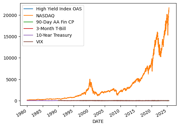
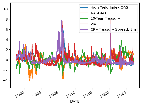
What does stationarity mean? See the the following plots. Some of these variable are stationary. Other are not? Why is this a problem?

df.plot()

<Axes: xlabel='DATE'>

df.info()

<class 'pandas.core.frame.DataFrame'>
DatetimeIndex: 11999 entries, 1980-01-01 to 2025-08-14
Data columns (total 6 columns):
 #   Column                Non-Null Count  Dtype  
---  ------                --------------  -----  
 0   High Yield Index OAS  7472 non-null   float64
 1   NASDAQ                11500 non-null  float64
 2   90-Day AA Fin CP      6606 non-null   float64
 3   3-Month T-Bill        11405 non-null  float64
 4   10-Year Treasury      11405 non-null  float64
 5   VIX                   8994 non-null   float64
dtypes: float64(6)
memory usage: 656.2 KB

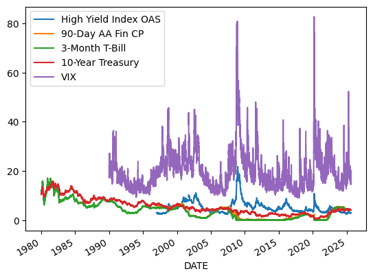
df.drop(columns=['NASDAQ']).plot()

<Axes: xlabel='DATE'>

Let’s try some transformations like those used in the OFR Financial Stress Index: https://www.financialresearch.gov/financial-stress-index/files/indicators/index.html

dfn = pd.DataFrame().reindex_like(df)
dfn

	High Yield Index OAS	NASDAQ	90-Day AA Fin CP	3-Month T-Bill	10-Year Treasury	VIX
DATE
1980-01-01	NaN	NaN	NaN	NaN	NaN	NaN
1980-01-02	NaN	NaN	NaN	NaN	NaN	NaN
1980-01-03	NaN	NaN	NaN	NaN	NaN	NaN
1980-01-04	NaN	NaN	NaN	NaN	NaN	NaN
1980-01-07	NaN	NaN	NaN	NaN	NaN	NaN
...	...	...	...	...	...	...
2025-08-08	NaN	NaN	NaN	NaN	NaN	NaN
2025-08-11	NaN	NaN	NaN	NaN	NaN	NaN
2025-08-12	NaN	NaN	NaN	NaN	NaN	NaN
2025-08-13	NaN	NaN	NaN	NaN	NaN	NaN
2025-08-14	NaN	NaN	NaN	NaN	NaN	NaN

11999 rows × 6 columns

df['NASDAQ'].rolling(250).mean()

DATE
1980-01-01   NaN
1980-01-02   NaN
1980-01-03   NaN
1980-01-04   NaN
1980-01-07   NaN
              ..
2025-08-08   NaN
2025-08-11   NaN
2025-08-12   NaN
2025-08-13   NaN
2025-08-14   NaN
Name: NASDAQ, Length: 11999, dtype: float64

df = df.dropna()

df['NASDAQ'].rolling(250).mean()

DATE
1997-01-02            NaN
1997-01-03            NaN
1997-01-06            NaN
1997-01-07            NaN
1997-01-08            NaN
                 ...     
2025-08-07    17255.97032
2025-08-08    17287.24620
2025-08-11    17318.88928
2025-08-12    17352.34916
2025-08-13    17386.03860
Name: NASDAQ, Length: 6585, dtype: float64

# 'High Yield Index OAS': Leave as is
dfn['High Yield Index OAS'] = df['High Yield Index OAS']
dfn['CP - Treasury Spread, 3m'] = df['90-Day AA Fin CP'] - df['3-Month T-Bill']
# 'NASDAQ':  # We're using something different, but still apply rolling mean transformation
dfn['NASDAQ'] = np.log(df['NASDAQ']) - np.log(df['NASDAQ'].rolling(250).mean())
dfn['10-Year Treasury'] = df['10-Year Treasury'] - df['10-Year Treasury'].rolling(250).mean()
# 'VIX': Leave as is
dfn['VIX'] = df['VIX']

dfn = dfn.drop(columns=['90-Day AA Fin CP', '3-Month T-Bill'])
dfn = dfn.dropna()

dfn.info()

<class 'pandas.core.frame.DataFrame'>
DatetimeIndex: 6336 entries, 1998-01-05 to 2025-08-13
Data columns (total 5 columns):
 #   Column                    Non-Null Count  Dtype  
---  ------                    --------------  -----  
 0   High Yield Index OAS      6336 non-null   float64
 1   NASDAQ                    6336 non-null   float64
 2   10-Year Treasury          6336 non-null   float64
 3   VIX                       6336 non-null   float64
 4   CP - Treasury Spread, 3m  6336 non-null   float64
dtypes: float64(5)
memory usage: 297.0 KB

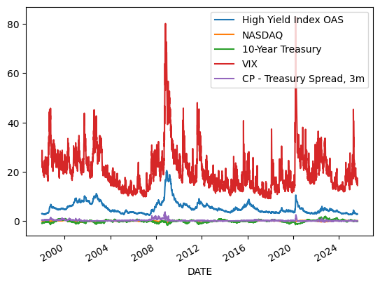
We finished with our transformations. Now, let’s normalize. First, why is it important?

dfn.plot()

<Axes: xlabel='DATE'>

Now, normalize each column, $\( z = \frac{x - \bar x}{\text{std}(x)} \)$

dfn = (dfn - dfn.mean()) / dfn.std()

dfn.plot()

<Axes: xlabel='DATE'>

def pca(dfn, module='scikitlearn'):
    if module == 'statsmodels':
        _pc1, _loadings, projection, rsquare, _, _, _ = statsmodels.multivariate.pca.pca(dfn,
            ncomp=1, standardize=True, demean=True, normalize=True, gls=False,
            weights=None, method='svd')
        _loadings = _loadings['comp_0']
        loadings = np.std(_pc1) * _loadings
        pc1 = _pc1 / np.std(_pc1)
        pc1 = pc1.rename(columns={'comp_0':'PC1'})['PC1']

    elif module == 'scikitlearn':
        pca = sklearn.decomposition.PCA(n_components=1)
        _pc1 = pd.Series(pca.fit_transform(dfn)[:,0], index=dfn.index, name='PC1')
        _loadings = pca.components_.T * np.sqrt(pca.explained_variance_)
        _loadings = pd.Series(_loadings[:,0], index=dfn.columns)

        loadings = np.std(_pc1) * _loadings
        pc1 = _pc1 / np.std(_pc1)
        pc1.name = 'PC1'
    else:
        raise ValueError



    loadings.name = "loadings"

    return pc1, loadings

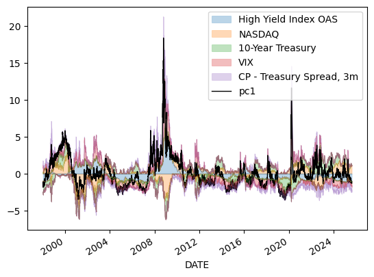
def stacked_plot(df, filename=None):
    """
    df=category_contributions
    # category_contributions.sum(axis=1).plot()
    """

    df_pos = df[df >= 0]
    df_neg = df[df < 0]

    alpha = .3
    linewidth = .5

    ax = df_pos.plot.area(alpha=alpha, linewidth=linewidth, legend=False)
    pc1 = df.sum(axis=1)
    pc1.name = 'pc1'
    pc1.plot(color="Black", label='pc1', linewidth=1)


    plt.legend()
    ax.set_prop_cycle(None)
    df_neg.plot.area(alpha=alpha, ax=ax, linewidth=linewidth, legend=False, ylim=(-3,3))
    # recompute the ax.dataLim
    ax.relim()
    # update ax.viewLim using the new dataLim
    ax.autoscale()
    # ax.set_ylabel('Standard Deviations')
    # ax.set_ylim(-3,4)
    # ax.set_ylim(-30,30)

    if not (filename is None):
        filename = Path(filename)
        figure = plt.gcf() # get current figure
        figure.set_size_inches(8, 6)
        plt.savefig(filename, dpi=300)

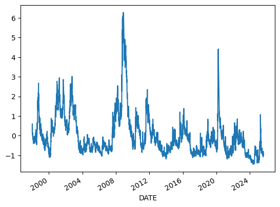
pc1, loadings = pca(dfn, module='scikitlearn')

pc1.plot()

<Axes: xlabel='DATE'>

stacked_plot(dfn)

Let’s compare solutions from two different packages

def root_mean_squared_error(sa, sb):
    return np.sqrt(np.mean((sa - sb)**2))

pc1_sk, loadings_sk = pca(dfn, module='scikitlearn')
pc1_sm, loadings_sm = pca(dfn, module='statsmodels')
root_mean_squared_error(pc1_sm, pc1_sk)

/opt/homebrew/Caskroom/mambaforge/base/envs/finm/lib/python3.13/site-packages/numpy/_core/fromnumeric.py:4062: FutureWarning: The behavior of DataFrame.std with axis=None is deprecated, in a future version this will reduce over both axes and return a scalar. To retain the old behavior, pass axis=0 (or do not pass axis)
  return std(axis=axis, dtype=dtype, out=out, ddof=ddof, **kwargs)

np.float64(4.679411434922667e-16)

Factor Analysis of a Panel of Stock Returns?

# Download sample data for multiple tickers
# Note: yfinance may return different structures depending on version and number of tickers
sample = yf.download("SPY AAPL MSFT", start="2017-01-01", end="2017-04-30", progress=False)

/var/folders/l3/tj6vb0ld2ys1h939jz0qrfrh0000gn/T/ipykernel_5885/673421897.py:3: FutureWarning: YF.download() has changed argument auto_adjust default to True
  sample = yf.download("SPY AAPL MSFT", start="2017-01-01", end="2017-04-30", progress=False)

# Let's examine the structure of the downloaded data
print("Sample columns:", sample.columns.tolist() if hasattr(sample, 'columns') else 'No columns attribute')
print("Sample shape:", sample.shape if hasattr(sample, 'shape') else 'No shape attribute')
if hasattr(sample, 'columns') and isinstance(sample.columns, pd.MultiIndex):
    print("Column levels:", sample.columns.levels)
    print("First level values:", sample.columns.levels[0].tolist())

Sample columns: [('Close', 'AAPL'), ('Close', 'MSFT'), ('Close', 'SPY'), ('High', 'AAPL'), ('High', 'MSFT'), ('High', 'SPY'), ('Low', 'AAPL'), ('Low', 'MSFT'), ('Low', 'SPY'), ('Open', 'AAPL'), ('Open', 'MSFT'), ('Open', 'SPY'), ('Volume', 'AAPL'), ('Volume', 'MSFT'), ('Volume', 'SPY')]
Sample shape: (81, 15)
Column levels: [['Close', 'High', 'Low', 'Open', 'Volume'], ['AAPL', 'MSFT', 'SPY']]
First level values: ['Close', 'High', 'Low', 'Open', 'Volume']

sample

Price	Close			High			Low			Open			Volume
Ticker	AAPL	MSFT	SPY	AAPL	MSFT	SPY	AAPL	MSFT	SPY	AAPL	MSFT	SPY	AAPL	MSFT	SPY
Date
2017-01-03	26.796825	56.497421	196.117371	26.838353	56.732149	196.631083	26.476140	56.091159	194.933213	26.716078	56.687009	195.943219	115127600	20694100	91366500
2017-01-04	26.766844	56.244614	197.284134	26.879892	56.650876	197.432152	26.704553	56.082109	196.439550	26.727624	56.407118	196.448252	84472400	21340000	78744400
2017-01-05	26.902958	56.244614	197.127396	26.960635	56.569623	197.284129	26.718390	56.000856	196.326349	26.743768	56.145305	197.014213	88774400	24876000	78379000
2017-01-06	27.202881	56.732140	197.832642	27.260558	57.012010	198.302816	26.870660	56.009898	196.692008	26.942179	56.244625	197.240556	127007600	19922900	71559900
2017-01-09	27.452047	56.551567	197.179642	27.553560	56.948803	197.710772	27.209804	56.461288	197.144806	27.212110	56.659902	197.571456	134247600	20382700	46939700
...	...	...	...	...	...	...	...	...	...	...	...	...	...	...	...
2017-04-24	33.282696	61.335896	207.403244	33.354525	61.453976	207.613127	33.176108	60.945336	205.120820	33.250257	61.290486	207.411984	68537200	29770000	119209900
2017-04-25	33.488934	61.690125	208.610046	33.574665	61.799120	208.959838	33.336005	61.399476	207.962918	33.345275	61.671962	208.050372	75486000	30242700	76698300
2017-04-26	33.291969	61.608391	208.478851	33.505145	62.044360	209.467031	33.222459	61.417654	208.435137	33.475022	61.835460	208.575046	80164800	26190800	84702500
2017-04-27	33.317463	62.008022	208.653793	33.403198	62.107933	208.959858	33.206243	61.381316	208.111599	33.347586	61.899034	208.802455	56985200	34971000	57410300
2017-04-28	33.285015	62.180584	208.199036	33.435628	62.798212	208.942346	33.196968	61.481214	208.067854	33.386968	62.589312	208.916112	83441600	39548800	63532800

81 rows × 15 columns

# When downloading multiple tickers, yfinance returns a DataFrame with MultiIndex columns
# The first level is the data type (e.g., 'Adj Close'), the second level is the ticker
# Display the adjusted close prices for all tickers
adj_close_data = sample['Adj Close'] if 'Adj Close' in sample.columns.get_level_values(0) else sample
adj_close_data

Price	Close			High			Low			Open			Volume
Ticker	AAPL	MSFT	SPY	AAPL	MSFT	SPY	AAPL	MSFT	SPY	AAPL	MSFT	SPY	AAPL	MSFT	SPY
Date
2017-01-03	26.796825	56.497421	196.117371	26.838353	56.732149	196.631083	26.476140	56.091159	194.933213	26.716078	56.687009	195.943219	115127600	20694100	91366500
2017-01-04	26.766844	56.244614	197.284134	26.879892	56.650876	197.432152	26.704553	56.082109	196.439550	26.727624	56.407118	196.448252	84472400	21340000	78744400
2017-01-05	26.902958	56.244614	197.127396	26.960635	56.569623	197.284129	26.718390	56.000856	196.326349	26.743768	56.145305	197.014213	88774400	24876000	78379000
2017-01-06	27.202881	56.732140	197.832642	27.260558	57.012010	198.302816	26.870660	56.009898	196.692008	26.942179	56.244625	197.240556	127007600	19922900	71559900
2017-01-09	27.452047	56.551567	197.179642	27.553560	56.948803	197.710772	27.209804	56.461288	197.144806	27.212110	56.659902	197.571456	134247600	20382700	46939700
...	...	...	...	...	...	...	...	...	...	...	...	...	...	...	...
2017-04-24	33.282696	61.335896	207.403244	33.354525	61.453976	207.613127	33.176108	60.945336	205.120820	33.250257	61.290486	207.411984	68537200	29770000	119209900
2017-04-25	33.488934	61.690125	208.610046	33.574665	61.799120	208.959838	33.336005	61.399476	207.962918	33.345275	61.671962	208.050372	75486000	30242700	76698300
2017-04-26	33.291969	61.608391	208.478851	33.505145	62.044360	209.467031	33.222459	61.417654	208.435137	33.475022	61.835460	208.575046	80164800	26190800	84702500
2017-04-27	33.317463	62.008022	208.653793	33.403198	62.107933	208.959858	33.206243	61.381316	208.111599	33.347586	61.899034	208.802455	56985200	34971000	57410300
2017-04-28	33.285015	62.180584	208.199036	33.435628	62.798212	208.942346	33.196968	61.481214	208.067854	33.386968	62.589312	208.916112	83441600	39548800	63532800

81 rows × 15 columns

tickers = [
    'AAPL','ABBV','ABT','ACN','ADP','ADSK','AES','AET','AFL','AMAT','AMGN','AMZN','APA',
    'APHA','APD','APTV','ARE','ASML','ATVI','AXP','BA','BAC','BAX','BDX','BIIB','BK',
    'BKNG','BMY','BRKB','BRK.A','COG','COST','CPB','CRM','CSCO','CVS','DAL','DD','DHR',
    'DIS','DOW','DUK','EMR','EPD','EQT','ESRT','EXPD','FFIV','FLS','FLT','FRT','GE',
    'GILD','GOOGL','GOOG','GS','HAL','HD','HON','IBM','INTC','IP','JNJ','JPM','KEY',
    'KHC','KIM','KO','LLY','LMT','LOW','MCD','MCHP','MDT','MMM','MO','MRK','MSFT',
    'MTD','NEE','NFLX','NKE','NOV','ORCL','OXY','PEP','PFE','PG','RTN','RTX','SBUX',
    'SHW','SLB','SO','SPG','STT','T','TGT','TXN','UNH','UPS','USB','UTX','V','VZ',
    'WMT','XOM',
]

all_tickers = " ".join(tickers)
all_tickers

'AAPL ABBV ABT ACN ADP ADSK AES AET AFL AMAT AMGN AMZN APA APHA APD APTV ARE ASML ATVI AXP BA BAC BAX BDX BIIB BK BKNG BMY BRKB BRK.A COG COST CPB CRM CSCO CVS DAL DD DHR DIS DOW DUK EMR EPD EQT ESRT EXPD FFIV FLS FLT FRT GE GILD GOOGL GOOG GS HAL HD HON IBM INTC IP JNJ JPM KEY KHC KIM KO LLY LMT LOW MCD MCHP MDT MMM MO MRK MSFT MTD NEE NFLX NKE NOV ORCL OXY PEP PFE PG RTN RTX SBUX SHW SLB SO SPG STT T TGT TXN UNH UPS USB UTX V VZ WMT XOM'

data = yf.download(all_tickers, start="1980-01-01", end=pd.to_datetime('today'), progress=False)

/var/folders/l3/tj6vb0ld2ys1h939jz0qrfrh0000gn/T/ipykernel_5885/3096157927.py:1: FutureWarning: YF.download() has changed argument auto_adjust default to True
  data = yf.download(all_tickers, start="1980-01-01", end=pd.to_datetime('today'), progress=False)

9 Failed downloads:

['BRK.A', 'FLT', 'COG', 'APHA', 'RTN', 'UTX', 'BRKB', 'ATVI']: YFTzMissingError('possibly delisted; no timezone found')

['MRK']: Timeout('Failed to perform, curl: (28) Connection timed out after 10002 milliseconds. See https://curl.se/libcurl/c/libcurl-errors.html first for more details.')

data

Price	Adj Close									Close	...	Volume
Ticker	APHA	ATVI	BRK.A	BRKB	COG	FLT	MRK	RTN	UTX	AAPL	...	TGT	TXN	UNH	UPS	USB	UTX	V	VZ	WMT	XOM
Date
1980-01-02	NaN	NaN	NaN	NaN	NaN	NaN	NaN	NaN	NaN	NaN	...	3691200	3796800.0	NaN	NaN	21600.0	NaN	NaN	NaN	2073600.0	6622400.0
1980-01-03	NaN	NaN	NaN	NaN	NaN	NaN	NaN	NaN	NaN	NaN	...	1468800	3134400.0	NaN	NaN	39600.0	NaN	NaN	NaN	4608000.0	7222400.0
1980-01-04	NaN	NaN	NaN	NaN	NaN	NaN	NaN	NaN	NaN	NaN	...	3206400	1195200.0	NaN	NaN	10800.0	NaN	NaN	NaN	2764800.0	4780800.0
1980-01-07	NaN	NaN	NaN	NaN	NaN	NaN	NaN	NaN	NaN	NaN	...	422400	2068800.0	NaN	NaN	36000.0	NaN	NaN	NaN	1228800.0	8331200.0
1980-01-08	NaN	NaN	NaN	NaN	NaN	NaN	NaN	NaN	NaN	NaN	...	451200	5414400.0	NaN	NaN	72000.0	NaN	NaN	NaN	5913600.0	8048000.0
...	...	...	...	...	...	...	...	...	...	...	...	...	...	...	...	...	...	...	...	...	...
2025-08-11	NaN	NaN	NaN	NaN	NaN	NaN	NaN	NaN	NaN	227.179993	...	5020200	6457800.0	11779500.0	8701400.0	7201900.0	NaN	5715800.0	12914900.0	12856700.0	13570700.0
2025-08-12	NaN	NaN	NaN	NaN	NaN	NaN	NaN	NaN	NaN	229.649994	...	6593800	9961500.0	12171800.0	7308600.0	8836600.0	NaN	5682800.0	12469300.0	17915300.0	14109400.0
2025-08-13	NaN	NaN	NaN	NaN	NaN	NaN	NaN	NaN	NaN	233.330002	...	7364700	4966300.0	19480300.0	13633200.0	10438100.0	NaN	5693400.0	14327700.0	19398500.0	17958700.0
2025-08-14	NaN	NaN	NaN	NaN	NaN	NaN	NaN	NaN	NaN	232.779999	...	4985000	3916400.0	22987500.0	12455700.0	6181100.0	NaN	6223200.0	10580600.0	10851800.0	13677600.0
2025-08-15	NaN	NaN	NaN	NaN	NaN	NaN	NaN	NaN	NaN	231.294998	...	4576323	NaN	61957831.0	NaN	NaN	NaN	NaN	NaN	NaN	NaN

11500 rows × 544 columns

data['Close']['AAPL'].plot()

<Axes: xlabel='Date'>

cols_with_many_nas = [
    "BRK.A",
    "APHA",
    "UTX",
    "RTN",
    "COG",
    "BRKB",
    "ATVI",
    "FLT",
    "DOW",
    "KHC",
    "V",
    "APTV",
    "ABBV",
    "ESRT",
]
df = data['Close']
print(f"Initial shape: {df.shape}")
df = df.drop(columns=cols_with_many_nas, errors='ignore')
print(f"After dropping columns: {df.shape}")
df = df.dropna()
print(f"After first dropna: {df.shape}")
df = df.pct_change()
print(f"After pct_change: {df.shape}")
df = df.dropna()
print(f"Final shape: {df.shape}")

# If DataFrame is empty, use a smaller date range or fewer tickers
if df.empty:
    print("DataFrame is empty! Trying with fewer tickers and recent data...")
    simple_tickers = ['AAPL', 'MSFT', 'GOOGL', 'AMZN', 'TSLA']
    data = yf.download(" ".join(simple_tickers), start="2020-01-01", end=pd.to_datetime('today'), progress=False)
    df = data['Close'].pct_change().dropna()
    print(f"New shape with simple tickers: {df.shape}")

Initial shape: (11500, 107)
After dropping columns: (11500, 93)
After first dropna: (0, 93)
After pct_change: (0, 93)
Final shape: (0, 93)
DataFrame is empty! Trying with fewer tickers and recent data...

/var/folders/l3/tj6vb0ld2ys1h939jz0qrfrh0000gn/T/ipykernel_5885/809774618.py:32: FutureWarning: YF.download() has changed argument auto_adjust default to True
  data = yf.download(" ".join(simple_tickers), start="2020-01-01", end=pd.to_datetime('today'), progress=False)

New shape with simple tickers: (1412, 5)

df.columns

Index(['AAPL', 'AMZN', 'GOOGL', 'MSFT', 'TSLA'], dtype='object', name='Ticker')

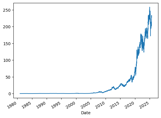
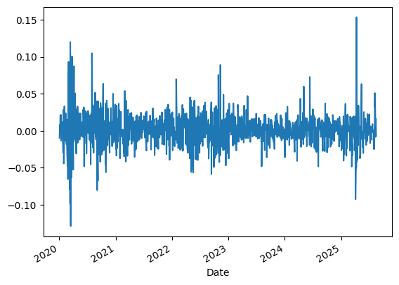
df['AAPL'].plot()

<Axes: xlabel='Date'>

if not df.empty:
    pc1, loadings = pca(df, module='scikitlearn')
    print(f"PCA completed successfully. PC1 shape: {pc1.shape}")
else:
    print("Cannot run PCA on empty DataFrame!")
    pc1 = pd.Series(dtype=float)
    loadings = pd.Series(dtype=float)

PCA completed successfully. PC1 shape: (1412,)

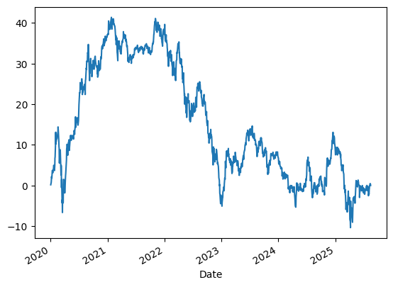
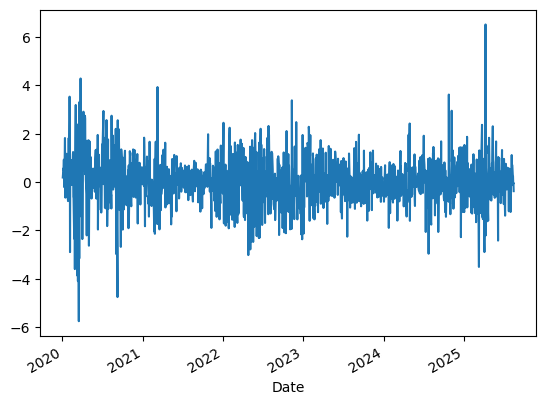
if not pc1.empty:
    pc1.plot()
else:
    print("No data to plot for PC1")

if not pc1.empty:
    pc1.cumsum().plot()
else:
    print("No data to plot for cumulative PC1")