3.3 Exploring CRSP Data with Python#
This script demonstrates how to explore and analyze CRSP daily stock data using various Python plotting libraries.
Overview#
We’ll analyze CRSP daily stock data for selected stocks (AAPL, JNJ, TSLA) and compare their performance against the S&P 500 index. The analysis includes:
Cumulative returns comparison
Dividend analysis
Rolling volatility analysis
Multiple plotting approaches (Matplotlib, Seaborn, Plotly)
Data Source#
CRSP Daily Stock File v2 (DSF) via WRDS
Filtered for common stock universe with proper exchange and trading filters
Date range: 2019-2025
import pandas as pd
import numpy as np
import wrds
import matplotlib.pyplot as plt
import seaborn as sns
import plotly.express as px
import plotly.graph_objects as go
from plotly.subplots import make_subplots
from datetime import datetime, timedelta

import config

DATA_DIR = config.DATA_DIR
WRDS_USERNAME = config.WRDS_USERNAME

db = wrds.Connection(wrds_username=WRDS_USERNAME)
Loading library list...
Done
Understanding CRSP Data Structure#
To find the right table, we use a combination of the web query interface and the SAS Studio explorer. The web query interface is available at: https://wrds-www.wharton.upenn.edu/pages/get-data/center-research-security-prices-crsp/annual-update/stock-version-2/daily-stock-file/
Note: Web queries often use merges of tables from many different sources. The results of these merges are not usually available through the Python API interface. Often, you’ll have to merge the tables yourself.
However, in this case, we can use the SAS Studio explorer to find the right table. Lucky for us, the data in the web query is available in a pre-merged table available through the Python API.
# First, let's look at the standard daily stock file (DSF) from the CIZ format
dsf = db.get_table(library="crsp", table="dsf_v2", obs=10)
dsf.head()
| permno | hdrcusip | permco | siccd | nasdissuno | yyyymmdd | sharetype | securitytype | securitysubtype | usincflg | ... | dlyopen | dlynumtrd | dlymmcnt | dlyprcvol | dlycumfacpr | dlycumfacshr | cusip | ticker | exchangetier | shrout | |
|---|---|---|---|---|---|---|---|---|---|---|---|---|---|---|---|---|---|---|---|---|---|
| 0 | 10000 | 68391610 | 7952 | 3990 | 10396 | 19860107 | NS | EQTY | COM | Y | ... | <NA> | <NA> | 9 | 2562.5 | 1.0 | 1.0 | 68391610 | OMFGA | SC1 | 3680 |
| 1 | 10000 | 68391610 | 7952 | 3990 | 10396 | 19860108 | NS | EQTY | COM | Y | ... | <NA> | <NA> | 9 | 32000.0 | 1.0 | 1.0 | 68391610 | OMFGA | SC1 | 3680 |
| 2 | 10000 | 68391610 | 7952 | 3990 | 10396 | 19860109 | NS | EQTY | COM | Y | ... | <NA> | <NA> | 9 | 3500.0 | 1.0 | 1.0 | 68391610 | OMFGA | SC1 | 3680 |
| 3 | 10000 | 68391610 | 7952 | 3990 | 10396 | 19860110 | NS | EQTY | COM | Y | ... | <NA> | <NA> | 10 | 21250.0 | 1.0 | 1.0 | 68391610 | OMFGA | SC1 | 3680 |
| 4 | 10000 | 68391610 | 7952 | 3990 | 10396 | 19860113 | NS | EQTY | COM | Y | ... | <NA> | <NA> | 10 | 14306.3 | 1.0 | 1.0 | 68391610 | OMFGA | SC1 | 3680 |
5 rows × 50 columns
dsf.info()
<class 'pandas.core.frame.DataFrame'>
RangeIndex: 10 entries, 0 to 9
Data columns (total 50 columns):
 #   Column            Non-Null Count  Dtype
---  ------            --------------  -----
 0   permno            10 non-null     Int64
 1   hdrcusip          10 non-null     string
 2   permco            10 non-null     Int64
 3   siccd             10 non-null     Int64
 4   nasdissuno        10 non-null     Int64
 5   yyyymmdd          10 non-null     Int64
 6   sharetype         10 non-null     string
 7   securitytype      10 non-null     string
 8   securitysubtype   10 non-null     string
 9   usincflg          10 non-null     string
 10  issuertype        10 non-null     string
 11  primaryexch       10 non-null     string
 12  conditionaltype   10 non-null     string
 13  tradingstatusflg  10 non-null     string
 14  dlycaldt          10 non-null     string
 15  dlydelflg         10 non-null     string
 16  dlyprc            10 non-null     Float64
 17  dlyprcflg         10 non-null     string
 18  dlycap            10 non-null     Float64
 19  dlycapflg         10 non-null     string
 20  dlyprevprc        9 non-null      Float64
 21  dlyprevprcflg     10 non-null     string
 22  dlyprevdt         9 non-null      string
 23  dlyprevcap        9 non-null      Float64
 24  dlyprevcapflg     10 non-null     string
 25  dlyret            9 non-null      Float64
 26  dlyretx           9 non-null      Float64
 27  dlyreti           9 non-null      Float64
 28  dlyretmissflg     10 non-null     string
 29  dlyretdurflg      10 non-null     string
 30  dlyorddivamt      10 non-null     Float64
 31  dlynonorddivamt   10 non-null     Float64
 32  dlyfacprc         10 non-null     Float64
 33  dlydistretflg     10 non-null     string
 34  dlyvol            10 non-null     Float64
 35  dlyclose          0 non-null      string
 36  dlylow            0 non-null      string
 37  dlyhigh           0 non-null      string
 38  dlybid            10 non-null     Float64
 39  dlyask            10 non-null     Float64
 40  dlyopen           0 non-null      string
 41  dlynumtrd         0 non-null      string
 42  dlymmcnt          10 non-null     Int64
 43  dlyprcvol         10 non-null     Float64
 44  dlycumfacpr       10 non-null     Float64
 45  dlycumfacshr      10 non-null     Float64
 46  cusip             10 non-null     string
 47  ticker            10 non-null     string
 48  exchangetier      10 non-null     string
 49  shrout            10 non-null     Int64
dtypes: Float64(16), Int64(7), string(27)
memory usage: 4.3 KB
Finding the Pre-merged Table#
Now, let’s find the pre-merged table that contains the data we want. Notice that it corresponds to the web query we used above.
df = db.get_table(library="crsp", table="wrds_dsfv2_query", obs=10)
df.head()
| permno | secinfostartdt | secinfoenddt | securitybegdt | securityenddt | securityhdrflg | hdrcusip | hdrcusip9 | cusip | cusip9 | ... | disrecorddt | dispaydt | dispermno | dispermco | disamountsourcetype | vwretd | vwretx | ewretd | ewretx | sprtrn | |
|---|---|---|---|---|---|---|---|---|---|---|---|---|---|---|---|---|---|---|---|---|---|
| 0 | 10000 | 1986-01-07 | 1986-12-03 | 1986-01-07 | 1987-06-11 | N | 68391610 | 683916100 | 68391610 | 683916100 | ... | <NA> | <NA> | <NA> | <NA> | <NA> | 0.013809 | 0.0138 | 0.011061 | 0.011046 | 0.014954 |
| 1 | 10000 | 1986-01-07 | 1986-12-03 | 1986-01-07 | 1987-06-11 | N | 68391610 | 683916100 | 68391610 | 683916100 | ... | <NA> | <NA> | <NA> | <NA> | <NA> | -0.020744 | -0.02075 | -0.005117 | -0.005135 | -0.027269 |
| 2 | 10000 | 1986-01-07 | 1986-12-03 | 1986-01-07 | 1987-06-11 | N | 68391610 | 683916100 | 68391610 | 683916100 | ... | <NA> | <NA> | <NA> | <NA> | <NA> | -0.011219 | -0.011315 | -0.011588 | -0.01166 | -0.008944 |
| 3 | 10000 | 1986-01-07 | 1986-12-03 | 1986-01-07 | 1987-06-11 | N | 68391610 | 683916100 | 68391610 | 683916100 | ... | <NA> | <NA> | <NA> | <NA> | <NA> | 0.000083 | 0.000047 | 0.003651 | 0.003632 | -0.000728 |
| 4 | 10000 | 1986-01-07 | 1986-12-03 | 1986-01-07 | 1987-06-11 | N | 68391610 | 683916100 | 68391610 | 683916100 | ... | <NA> | <NA> | <NA> | <NA> | <NA> | 0.00275 | 0.00268 | 0.002433 | 0.002369 | 0.00369 |
5 rows × 98 columns
Note: We actually just made a mistake above. For some reason, we aren’t allowed to access this via “crspa”, but we are via “crsp”.
df.info()
<class 'pandas.core.frame.DataFrame'>
RangeIndex: 10 entries, 0 to 9
Data columns (total 98 columns):
 #   Column               Non-Null Count  Dtype
---  ------               --------------  -----
 0   permno               10 non-null     Int64
 1   secinfostartdt       10 non-null     string
 2   secinfoenddt         10 non-null     string
 3   securitybegdt        10 non-null     string
 4   securityenddt        10 non-null     string
 5   securityhdrflg       10 non-null     string
 6   hdrcusip             10 non-null     string
 7   hdrcusip9            10 non-null     string
 8   cusip                10 non-null     string
 9   cusip9               10 non-null     string
 10  primaryexch          10 non-null     string
 11  conditionaltype      10 non-null     string
 12  exchangetier         10 non-null     string
 13  tradingstatusflg     10 non-null     string
 14  securitynm           10 non-null     string
 15  shareclass           10 non-null     string
 16  usincflg             10 non-null     string
 17  issuertype           10 non-null     string
 18  securitytype         10 non-null     string
 19  securitysubtype      10 non-null     string
 20  sharetype            10 non-null     string
 21  securityactiveflg    10 non-null     string
 22  delactiontype        10 non-null     string
 23  delstatustype        10 non-null     string
 24  delreasontype        10 non-null     string
 25  delpaymenttype       10 non-null     string
 26  ticker               10 non-null     string
 27  tradingsymbol        10 non-null     string
 28  permco               10 non-null     Int64
 29  siccd                10 non-null     Int64
 30  naics                10 non-null     string
 31  icbindustry          10 non-null     string
 32  uesindustry          10 non-null     string
 33  nasdcompno           10 non-null     Int64
 34  nasdissuno           10 non-null     Int64
 35  issuernm             10 non-null     string
 36  yyyymmdd             10 non-null     Int64
 37  dlycaldt             10 non-null     string
 38  dlydelflg            10 non-null     string
 39  dlyprc               10 non-null     Float64
 40  dlyprcflg            10 non-null     string
 41  dlycap               10 non-null     Float64
 42  dlycapflg            10 non-null     string
 43  dlyprevprc           9 non-null      Float64
 44  dlyprevprcflg        10 non-null     string
 45  dlyprevdt            9 non-null      string
 46  dlyprevcap           9 non-null      Float64
 47  dlyprevcapflg        10 non-null     string
 48  dlyret               9 non-null      Float64
 49  dlyretx              9 non-null      Float64
 50  dlyreti              9 non-null      Float64
 51  dlyretmissflg        10 non-null     string
 52  dlyretdurflg         10 non-null     string
 53  dlyorddivamt         10 non-null     Float64
 54  dlynonorddivamt      10 non-null     Float64
 55  dlyfacprc            10 non-null     Float64
 56  dlydistretflg        10 non-null     string
 57  dlyvol               10 non-null     Float64
 58  dlyclose             0 non-null      string
 59  dlylow               0 non-null      string
 60  dlyhigh              0 non-null      string
 61  dlybid               10 non-null     Float64
 62  dlyask               10 non-null     Float64
 63  dlyopen              0 non-null      string
 64  dlynumtrd            0 non-null      string
 65  dlymmcnt             10 non-null     Int64
 66  dlyprcvol            10 non-null     Float64
 67  shrstartdt           10 non-null     string
 68  shrenddt             10 non-null     string
 69  shrout               10 non-null     Int64
 70  shrsource            10 non-null     string
 71  shrfactype           10 non-null     string
 72  shradrflg            10 non-null     string
 73  dlycumfacpr          10 non-null     Float64
 74  dlycumfacshr         10 non-null     Float64
 75  disexdt              0 non-null      string
 76  disseqnbr            0 non-null      string
 77  disordinaryflg       0 non-null      string
 78  distype              0 non-null      string
 79  disfreqtype          0 non-null      string
 80  dispaymenttype       0 non-null      string
 81  disdetailtype        0 non-null      string
 82  distaxtype           0 non-null      string
 83  disorigcurtype       0 non-null      string
 84  disdivamt            0 non-null      string
 85  disfacpr             0 non-null      string
 86  disfacshr            0 non-null      string
 87  disdeclaredt         0 non-null      string
 88  disrecorddt          0 non-null      string
 89  dispaydt             0 non-null      string
 90  dispermno            0 non-null      string
 91  dispermco            0 non-null      string
 92  disamountsourcetype  0 non-null      string
 93  vwretd               10 non-null     Float64
 94  vwretx               10 non-null     Float64
 95  ewretd               10 non-null     Float64
 96  ewretx               10 non-null     Float64
 97  sprtrn               10 non-null     Float64
dtypes: Float64(21), Int64(8), string(69)
memory usage: 8.1 KB
Notice that this now matches the web query variables list.
Defining the Data Query#
Now, let’s explore some of the columns. But first, we need to download more data.
query = """
SELECT
    permno,
    permco,
    dlycaldt,
    issuertype,
    securitytype,
    securitysubtype,
    sharetype,
    usincflg,
    primaryexch,
    conditionaltype,
    tradingstatusflg,
    dlyret,
    dlyretx,
    dlyreti,
    dlyorddivamt,
    dlynonorddivamt,
    shrout,
    dlyprc,
    ticker,
    securitynm,
    sprtrn,
    vwretd
FROM
    crsp.wrds_dsfv2_query
WHERE
    dlycaldt between '01/01/2019' and '01/01/2025' AND
    sharetype = 'NS' AND
    securitytype = 'EQTY' AND
    securitysubtype = 'COM' AND
    usincflg = 'Y' AND
    issuertype IN ('ACOR', 'CORP') AND
    primaryexch IN ('N', 'A', 'Q') AND
    conditionaltype = 'RW' AND
    tradingstatusflg = 'A'
"""
def pull_crsp_sample(data_dir=DATA_DIR):
    """
    Pull CRSP daily stock data with comprehensive filtering for common stock universe.

    This function implements the equivalent of legacy CRSP filters:
    - shrcd = 10 or 11 (common stock)
    - exchcd = 1, 2, or 3 (NYSE, AMEX, NASDAQ)

    Filters applied:
    1. Date range: 2019-2025
    2. Common stock universe:
       - sharetype = 'NS' (New Shares)
       - securitytype = 'EQTY' (Equity)
       - securitysubtype = 'COM' (Common Stock)
       - usincflg = 'Y' (US Incorporated)
       - issuertype IN ('ACOR', 'CORP') (Accordion or Corporate)
    3. Exchange and trading filters:
       - primaryexch IN ('N', 'A', 'Q') (NYSE, AMEX, NASDAQ)
       - conditionaltype = 'RW' (Regular Way trading)
       - tradingstatusflg = 'A' (Active trading status)

    Caching:
    - Data is cached locally as a parquet file to avoid repeated WRDS queries
    - If cached data exists, it loads from disk instead of querying WRDS
    - If no cache exists, queries WRDS and saves the result for future use

    Args:
        data_dir: Directory to store/load cached data

    Returns:
        DataFrame: Filtered CRSP daily stock data
    """
    data_path = data_dir / "crsp_dsf_v2_example.parquet"
    if data_path.exists():
        df = pd.read_parquet(data_path)
    else:
        df = db.raw_sql(query, date_cols=["dlycaldt"])
        df.to_parquet(data_path)
    return df
df = pull_crsp_sample()
df.head()
| permno | permco | dlycaldt | issuertype | securitytype | securitysubtype | sharetype | usincflg | primaryexch | conditionaltype | ... | dlyretx | dlyreti | dlyorddivamt | dlynonorddivamt | shrout | dlyprc | ticker | securitynm | sprtrn | vwretd | |
|---|---|---|---|---|---|---|---|---|---|---|---|---|---|---|---|---|---|---|---|---|---|
| 0 | 10026 | 7976 | 2019-01-02 | CORP | EQTY | COM | NS | Y | Q | RW | ... | -0.024829 | 0.0 | 0.0 | 0.0 | 18774 | 141.0 | JJSF | J & J SNACK FOODS CORP; COM NONE; CONS | 0.001269 | 0.001796 |
| 1 | 10028 | 7978 | 2019-01-02 | CORP | EQTY | COM | NS | Y | A | RW | ... | -0.043488 | 0.0 | 0.0 | 0.0 | 26924 | 0.4399 | DGSE | D G S E COMPANIES INC; COM NONE; CONS | 0.001269 | 0.001796 |
| 2 | 10032 | 7980 | 2019-01-02 | CORP | EQTY | COM | NS | Y | Q | RW | ... | 0.012921 | 0.0 | 0.0 | 0.0 | 30992 | 51.74 | PLXS | PLEXUS CORP; COM NONE; CONS | 0.001269 | 0.001796 |
| 3 | 10044 | 7992 | 2019-01-02 | CORP | EQTY | COM | NS | Y | Q | RW | ... | 0.012887 | 0.0 | 0.0 | 0.0 | 5949 | 8.63 | RMCF | ROCKY MOUNTAIN CHOC FAC INC NEW; COM NONE; CONS | 0.001269 | 0.001796 |
| 4 | 10051 | 7999 | 2019-01-02 | CORP | EQTY | COM | NS | Y | N | RW | ... | -0.003694 | 0.0 | 0.0 | 0.0 | 36848 | 18.88 | HNGR | HANGER INC; COM NONE; CONS | 0.001269 | 0.001796 |
5 rows × 22 columns
df.info()
<class 'pandas.core.frame.DataFrame'>
Index: 5981476 entries, 0 to 481475
Data columns (total 22 columns):
 #   Column            Dtype
---  ------            -----
 0   permno            Int64
 1   permco            Int64
 2   dlycaldt          datetime64[ns]
 3   issuertype        string
 4   securitytype      string
 5   securitysubtype   string
 6   sharetype         string
 7   usincflg          string
 8   primaryexch       string
 9   conditionaltype   string
 10  tradingstatusflg  string
 11  dlyret            Float64
 12  dlyretx           Float64
 13  dlyreti           Float64
 14  dlyorddivamt      Float64
 15  dlynonorddivamt   Float64
 16  shrout            Int64
 17  dlyprc            Float64
 18  ticker            string
 19  securitynm        string
 20  sprtrn            Float64
 21  vwretd            Float64
dtypes: Float64(8), Int64(3), datetime64[ns](1), string(10)
memory usage: 1.1 GB
Data Summary and Exploration#
Let’s look at some summary statistics to understand our dataset.
# Let's look at some summary statistics
print("\n=== Data Summary ===")
print(f"Date range: {df['dlycaldt'].min()} to {df['dlycaldt'].max()}")
print(f"Number of unique stocks: {df['permno'].nunique()}")
print(f"Total observations: {len(df)}")
=== Data Summary ===
Date range: 2019-01-02 00:00:00 to 2024-12-31 00:00:00
Number of unique stocks: 5488
Total observations: 5981476
Identifying Well-Known Stocks#
We’ll look for stocks with recognizable tickers and good data coverage for our analysis.
# Let's identify some well-known stocks for analysis
# We'll look for stocks with recognizable tickers and good data coverage
stock_summary = df.groupby(['permno', 'ticker', 'securitynm']).agg({
    'dlycaldt': ['count', 'min', 'max'],
    'dlyret': 'count',
    'dlyorddivamt': lambda x: (x > 0).sum()
}).round(2)

stock_summary.columns = ['obs_count', 'start_date', 'end_date', 'return_obs', 'dividend_days']
stock_summary = stock_summary.reset_index()

# Filter for stocks with good data coverage and recognizable names
good_stocks = stock_summary[
    (stock_summary['obs_count'] > 500) &  # At least 500 observations
    (stock_summary['ticker'].notna()) &   # Has a ticker
    (stock_summary['ticker'] != '')       # Ticker is not empty
].sort_values('obs_count', ascending=False)

print("\n=== Top Stocks by Data Coverage ===")
good_stocks.head(20)
=== Top Stocks by Data Coverage ===
| permno | ticker | securitynm | obs_count | start_date | end_date | return_obs | dividend_days | |
|---|---|---|---|---|---|---|---|---|
| 4193 | 32651 | HL | HECLA MINING CO; COM NONE; CONS | 1526 | 2019-01-02 | 2024-12-31 | 1526 | 40.0 |
| 1624 | 17743 | WRB | BERKLEY W R CORP; COM NONE; CONS | 1520 | 2019-01-02 | 2024-12-31 | 1520 | 35.0 |
| 1240 | 16437 | CWH | CAMPING WORLD HOLDINGS INC; COM A; CONS | 1520 | 2019-01-02 | 2024-12-31 | 1520 | 34.0 |
| 1004 | 15540 | RILY | B RILEY FINANCIAL INC; COM NONE; CONS | 1519 | 2019-01-02 | 2024-12-31 | 1519 | 31.0 |
| 401 | 13641 | FANG | DIAMONDBACK ENERGY INC; COM NONE; CONS | 1519 | 2019-01-02 | 2024-12-31 | 1519 | 33.0 |
| 4195 | 32707 | HP | HELMERICH & PAYNE INC; COM NONE; CONS | 1518 | 2019-01-02 | 2024-12-31 | 1518 | 32.0 |
| 4337 | 47626 | CNA | C N A FINANCIAL CORP; COM NONE; CONS | 1516 | 2019-01-02 | 2024-12-31 | 1516 | 30.0 |
| 4697 | 76266 | PRK | PARK NATIONAL CORP; COM NONE; CONS | 1516 | 2019-01-02 | 2024-12-31 | 1516 | 30.0 |
| 4863 | 78211 | UVE | UNIVERSAL INSURANCE HOLDINGS INC; COM NONE; CONS | 1516 | 2019-01-02 | 2024-12-31 | 1516 | 30.0 |
| 70 | 10901 | ITIC | INVESTORS TITLE CO; COM NONE; CONS | 1516 | 2019-01-02 | 2024-12-31 | 1516 | 30.0 |
| 4040 | 25129 | CBSH | COMMERCE BANCSHARES INC; COM NONE; CONS | 1516 | 2019-01-02 | 2024-12-31 | 1516 | 30.0 |
| 4817 | 77584 | BKE | BUCKLE INC; COM NONE; CONS | 1516 | 2019-01-02 | 2024-12-31 | 1516 | 28.0 |
| 439 | 13802 | APAM | ARTISAN PARTNERS ASSET MGMT INC; COM A; CONS | 1516 | 2019-01-02 | 2024-12-31 | 1516 | 30.0 |
| 4556 | 65294 | RLI | R L I CORP; COM NONE; CONS | 1516 | 2019-01-02 | 2024-12-31 | 1516 | 30.0 |
| 427 | 13766 | BCC | BOISE CASCADE CO; COM NONE; CONS | 1516 | 2019-01-02 | 2024-12-31 | 1516 | 32.0 |
| 4208 | 34497 | NPK | NATIONAL PRESTO INDS INC; COM NONE; CONS | 1516 | 2019-01-02 | 2024-12-31 | 1516 | 12.0 |
| 5677 | 88341 | HWBK | HAWTHORN BANCSHARES INC; COM NONE; CONS | 1515 | 2019-01-02 | 2024-12-31 | 1515 | 29.0 |
| 5640 | 87725 | IIIN | INSTEEL INDUSTRIES INC; COM NONE; CONS | 1515 | 2019-01-02 | 2024-12-31 | 1515 | 29.0 |
| 168 | 12189 | HIFS | HINGHAM INSTITUTION FOR SVGS MA; COM NONE; CONS | 1515 | 2019-01-02 | 2024-12-31 | 1515 | 29.0 |
| 5582 | 87137 | DVN | DEVON ENERGY CORP NEW; COM NONE; CONS | 1515 | 2019-01-02 | 2024-12-31 | 1515 | 30.0 |
Selecting Stocks for Analysis#
Let’s select three stocks for analysis:
A dividend-paying stock (likely a utility or financial)
A growth stock that pays no dividends (likely tech)
A stock in between
# Let's look for some specific well-known stocks
target_tickers = ['AAPL', 'MSFT', 'JNJ', 'PG', 'KO', 'XOM', 'JPM', 'WMT', 'NVDA', 'TSLA']
available_stocks = good_stocks[good_stocks['ticker'].isin(target_tickers)]

print("\n=== Available Target Stocks ===")
available_stocks
=== Available Target Stocks ===
| permno | ticker | securitynm | obs_count | start_date | end_date | return_obs | dividend_days | |
|---|---|---|---|---|---|---|---|---|
| 3375 | 22111 | JNJ | JOHNSON & JOHNSON; COM NONE; CONS | 1510 | 2019-01-02 | 2024-12-31 | 1510 | 24.0 |
| 4430 | 55976 | WMT | WALMART INC; COM NONE; CONS | 1510 | 2019-01-02 | 2024-12-31 | 1510 | 24.0 |
| 4344 | 47896 | JPM | JPMORGAN CHASE & CO; COM NONE; CONS | 1510 | 2019-01-02 | 2024-12-31 | 1510 | 24.0 |
| 5516 | 86580 | NVDA | NVIDIA CORP; COM NONE; CONS | 1510 | 2019-01-02 | 2024-12-31 | 1510 | 24.0 |
| 6450 | 93436 | TSLA | TESLA INC; COM NONE; CONS | 1510 | 2019-01-02 | 2024-12-31 | 1510 | 0.0 |
| 141 | 11850 | XOM | EXXON MOBIL CORP; COM NONE; CONS | 1510 | 2019-01-02 | 2024-12-31 | 1510 | 24.0 |
| 682 | 14593 | AAPL | APPLE INC; COM NONE; CONS | 1510 | 2019-01-02 | 2024-12-31 | 1510 | 24.0 |
| 1792 | 18163 | PG | PROCTER & GAMBLE CO; COM NONE; CONS | 1510 | 2019-01-02 | 2024-12-31 | 1510 | 24.0 |
| 91 | 11308 | KO | COCA COLA CO; COM NONE; CONS | 1510 | 2019-01-02 | 2024-12-31 | 1510 | 24.0 |
| 8 | 10107 | MSFT | MICROSOFT CORP; COM NONE; CONS | 1510 | 2019-01-02 | 2024-12-31 | 1510 | 24.0 |
# Select three stocks for analysis
selected_stocks = ['AAPL', 'JNJ', 'TSLA']  # Apple (tech, some dividends), J&J (dividend payer), Tesla (no dividends)

# Filter data for selected stocks and market
selected_data = df[df['ticker'].isin(selected_stocks)].copy()
market_data = df[['dlycaldt', 'sprtrn', 'vwretd']].drop_duplicates().copy()
Data Quality Check#
Let’s verify our data quality and check for any duplicate entries.
# Debug: Check for duplicate dates in selected data
print(f"\n=== Data Quality Check ===")
print(f"Selected stocks data shape: {selected_data.shape}")
print(f"Duplicate ticker-date combinations: {selected_data.duplicated(subset=['ticker', 'dlycaldt']).sum()}")
print(f"Market data shape: {market_data.shape}")
print(f"Duplicate dates in market data: {market_data.duplicated(subset=['dlycaldt']).sum()}")

# Show sample of selected data
print(f"\nSample of selected data:")
print(selected_data[['ticker', 'dlycaldt', 'dlyret']].head(10))
=== Data Quality Check ===
Selected stocks data shape: (4530, 22)
Duplicate ticker-date combinations: 0
Market data shape: (1510, 3)
Duplicate dates in market data: 0

Sample of selected data:
      ticker   dlycaldt    dlyret
568     AAPL 2019-01-02  0.001141
1537     JNJ 2019-01-02 -0.010074
3592    TSLA 2019-01-02 -0.068149
4161    AAPL 2019-01-03 -0.099607
5129     JNJ 2019-01-03  -0.01589
7184    TSLA 2019-01-03 -0.031472
7754    AAPL 2019-01-04  0.042689
8721     JNJ 2019-01-04  0.016783
10776   TSLA 2019-01-04  0.057697
11345   AAPL 2019-01-07 -0.002226
Calculating Cumulative Returns#
Now let’s calculate cumulative returns for our selected stocks to analyze their performance over time.
def calculate_cumulative_returns(data, return_col='dlyret'):
    """Calculate cumulative returns for each stock"""
    data = data.copy()
    data = data.sort_values(['ticker', 'dlycaldt'])

    # Handle potential duplicate dates by taking the last observation for each ticker-date combination
    data = data.drop_duplicates(subset=['ticker', 'dlycaldt'], keep='last')

    # Calculate cumulative returns (1 + return) for each stock using a safer approach
    data['cumret'] = 1.0  # Initialize with 1

    for ticker in data['ticker'].unique():
        mask = data['ticker'] == ticker
        returns = data.loc[mask, return_col].fillna(0)
        cumulative = (1 + returns).cumprod()
        data.loc[mask, 'cumret'] = cumulative

    return data
# Calculate cumulative returns
stock_cumret = calculate_cumulative_returns(selected_data)
market_cumret = market_data.copy()
market_cumret['cumret'] = (1 + market_cumret['sprtrn']).cumprod()
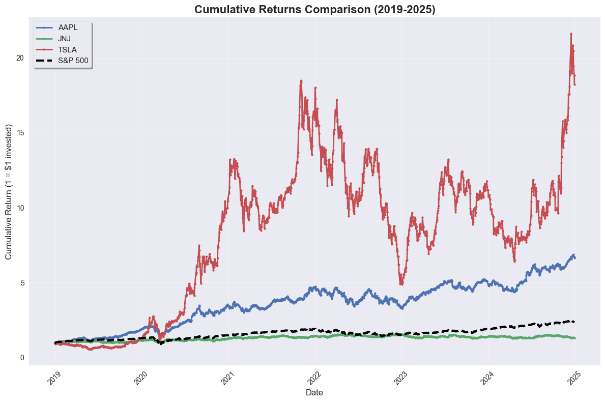
Plot 1: Matplotlib - Cumulative Returns Comparison#
Let’s start with a traditional matplotlib plot to visualize the cumulative returns.
# Plot 1: Matplotlib - Cumulative Returns Comparison
plt.figure(figsize=(12, 8))
plt.style.use('seaborn-v0_8')

for ticker in selected_stocks:
    ticker_data = stock_cumret[stock_cumret['ticker'] == ticker]
    plt.plot(ticker_data['dlycaldt'], ticker_data['cumret'],
             label=ticker, linewidth=2, marker='o', markersize=3)

# Add market portfolio
plt.plot(market_cumret['dlycaldt'], market_cumret['cumret'],
         label='S&P 500', linewidth=3, color='black', linestyle='--')

plt.title('Cumulative Returns Comparison (2019-2025)', fontsize=16, fontweight='bold')
plt.xlabel('Date', fontsize=12)
plt.ylabel('Cumulative Return (1 = $1 invested)', fontsize=12)
plt.legend(fontsize=11, frameon=True, fancybox=True, shadow=True)
plt.grid(True, alpha=0.3)
plt.xticks(rotation=45)
plt.tight_layout()
plt.show()
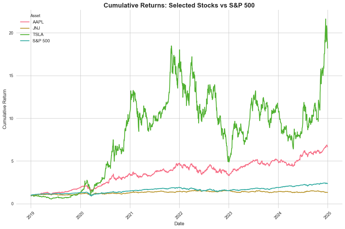
Plot 2: Seaborn - Cumulative Returns with Better Styling#
Now let’s use Seaborn for enhanced styling and aesthetics.
# Plot 2: Seaborn - Cumulative Returns with better styling
plt.figure(figsize=(12, 8))
sns.set_style("whitegrid")
sns.set_palette("husl")

# Prepare data for seaborn
plot_data = []
for ticker in selected_stocks:
    ticker_data = stock_cumret[stock_cumret['ticker'] == ticker][['dlycaldt', 'cumret']]
    ticker_data['ticker'] = ticker
    plot_data.append(ticker_data)

# Add market data
market_plot_data = market_cumret[['dlycaldt', 'cumret']].copy()
market_plot_data['ticker'] = 'S&P 500'
plot_data.append(market_plot_data)

plot_df = pd.concat(plot_data, ignore_index=True)

sns.lineplot(data=plot_df, x='dlycaldt', y='cumret', hue='ticker',
             linewidth=2, markers=True, markersize=4)

plt.title('Cumulative Returns: Selected Stocks vs S&P 500', fontsize=16, fontweight='bold')
plt.xlabel('Date', fontsize=12)
plt.ylabel('Cumulative Return', fontsize=12)
plt.legend(title='Asset', fontsize=11)
plt.xticks(rotation=45)
plt.tight_layout()
plt.show()
Plot 3: Plotly Express - Interactive Cumulative Returns#
Finally, let’s create an interactive plot using Plotly Express for enhanced user experience.
# Plot 3: Plotly Express - Interactive Cumulative Returns
fig = px.line(plot_df, x='dlycaldt', y='cumret', color='ticker',
              title='Interactive Cumulative Returns Comparison',
              labels={'dlycaldt': 'Date', 'cumret': 'Cumulative Return', 'ticker': 'Asset'},
              line_shape='linear', render_mode='svg')

fig.update_layout(
    title_font_size=16,
    xaxis_title_font_size=12,
    yaxis_title_font_size=12,
    legend_title_font_size=12,
    hovermode='x unified'
)

fig.show()
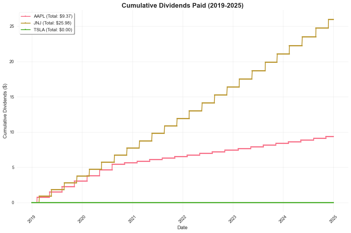
Dividend Analysis#
Now let’s analyze dividends to understand the income component of our selected stocks.
# Now let's analyze dividends
print("\n=== Dividend Analysis ===")
=== Dividend Analysis ===
def calculate_cumulative_dividends(data):
    """Calculate cumulative dividends for each stock"""
    data = data.copy()
    data = data.sort_values(['ticker', 'dlycaldt'])

    # Handle potential duplicate dates by taking the last observation for each ticker-date combination
    data = data.drop_duplicates(subset=['ticker', 'dlycaldt'], keep='last')

    # Sum up all dividend amounts (ordinary + non-ordinary)
    data['total_div'] = data['dlyorddivamt'].fillna(0) + data['dlynonorddivamt'].fillna(0)

    # Calculate cumulative dividends using a safer approach
    data['cumdiv'] = 0.0  # Initialize with 0

    for ticker in data['ticker'].unique():
        mask = data['ticker'] == ticker
        dividends = data.loc[mask, 'total_div']
        cumulative = dividends.cumsum()
        data.loc[mask, 'cumdiv'] = cumulative

    return data
# Calculate cumulative dividends
stock_cumdiv = calculate_cumulative_dividends(selected_data)

# Get dividend summary
div_summary = stock_cumdiv.groupby('ticker').agg({
    'total_div': ['sum', 'count'],
    'cumdiv': 'max'
}).round(4)

div_summary.columns = ['total_dividends', 'dividend_days', 'cumulative_dividends']
print(div_summary)
        total_dividends  dividend_days  cumulative_dividends
ticker
AAPL               9.37           1510                  9.37
JNJ               25.98           1510                 25.98
TSLA                0.0           1510                  0.00
Plot 4: Matplotlib - Cumulative Dividends#
Let’s visualize the cumulative dividends using matplotlib.
# Plot 4: Matplotlib - Cumulative Dividends
plt.figure(figsize=(12, 8))

for ticker in selected_stocks:
    ticker_data = stock_cumdiv[stock_cumdiv['ticker'] == ticker]
    plt.plot(ticker_data['dlycaldt'], ticker_data['cumdiv'],
             label=f'{ticker} (Total: ${ticker_data["cumdiv"].max():.2f})',
             linewidth=2, marker='s', markersize=3)

plt.title('Cumulative Dividends Paid (2019-2025)', fontsize=16, fontweight='bold')
plt.xlabel('Date', fontsize=12)
plt.ylabel('Cumulative Dividends ($)', fontsize=12)
plt.legend(fontsize=11, frameon=True, fancybox=True, shadow=True)
plt.grid(True, alpha=0.3)
plt.xticks(rotation=45)
plt.tight_layout()
plt.show()
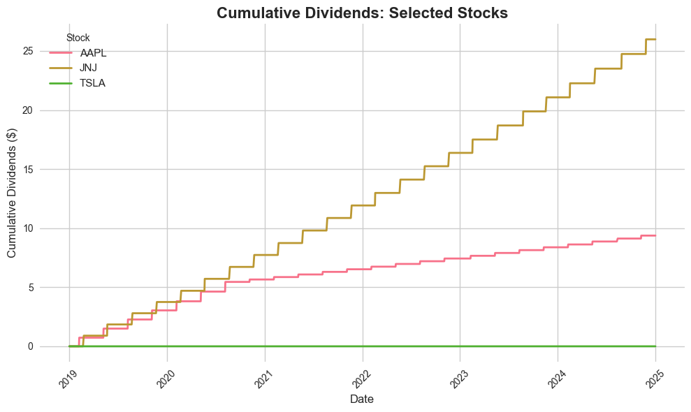
Plot 5: Seaborn - Dividend Comparison#
Now let’s use Seaborn for the dividend visualization.
# Plot 5: Seaborn - Dividend Comparison
plt.figure(figsize=(10, 6))
sns.set_style("whitegrid")

# Prepare dividend data for seaborn
div_plot_data = []
for ticker in selected_stocks:
    ticker_data = stock_cumdiv[stock_cumdiv['ticker'] == ticker][['dlycaldt', 'cumdiv']]
    ticker_data['ticker'] = ticker
    div_plot_data.append(ticker_data)

div_plot_df = pd.concat(div_plot_data, ignore_index=True)

sns.lineplot(data=div_plot_df, x='dlycaldt', y='cumdiv', hue='ticker',
             linewidth=2, markers=True, markersize=4)

plt.title('Cumulative Dividends: Selected Stocks', fontsize=16, fontweight='bold')
plt.xlabel('Date', fontsize=12)
plt.ylabel('Cumulative Dividends ($)', fontsize=12)
plt.legend(title='Stock', fontsize=11)
plt.xticks(rotation=45)
plt.tight_layout()
plt.show()
Plot 6: Plotly Express - Interactive Dividends#
Let’s create an interactive dividend plot with Plotly.
# Plot 6: Plotly Express - Interactive Dividends
fig = px.line(div_plot_df, x='dlycaldt', y='cumdiv', color='ticker',
              title='Interactive Cumulative Dividends',
              labels={'dlycaldt': 'Date', 'cumdiv': 'Cumulative Dividends ($)', 'ticker': 'Stock'},
              line_shape='linear', render_mode='svg')

fig.update_layout(
    title_font_size=16,
    xaxis_title_font_size=12,
    yaxis_title_font_size=12,
    legend_title_font_size=12,
    hovermode='x unified'
)

fig.show()
Rolling Volatility Analysis#
Now let’s analyze the rolling volatility of our selected stocks to understand their risk characteristics over time.
# Now let's calculate rolling volatility (3-month window)
print("\n=== Rolling Volatility Analysis ===")
=== Rolling Volatility Analysis ===
def calculate_rolling_volatility(data, window_days=63):  # ~3 months (63 trading days)
    """Calculate rolling volatility for each stock"""
    data = data.copy()
    data = data.sort_values(['ticker', 'dlycaldt'])

    # Handle potential duplicate dates by taking the last observation for each ticker-date combination
    data = data.drop_duplicates(subset=['ticker', 'dlycaldt'], keep='last')

    # Calculate rolling standard deviation of returns using a safer approach
    data['rolling_vol'] = np.nan
    data['rolling_vol_annual'] = np.nan

    for ticker in data['ticker'].unique():
        mask = data['ticker'] == ticker
        returns = data.loc[mask, 'dlyret'].fillna(0)

        # Calculate rolling standard deviation
        rolling_std = returns.rolling(window=window_days, min_periods=30).std()
        data.loc[mask, 'rolling_vol'] = rolling_std

        # Annualize volatility (multiply by sqrt(252) for daily data)
        data.loc[mask, 'rolling_vol_annual'] = rolling_std * np.sqrt(252)

    return data
# Calculate rolling volatility for stocks
stock_vol = calculate_rolling_volatility(selected_data)

# Calculate rolling volatility for market
market_vol = market_data.copy()
market_vol['rolling_vol'] = market_vol['sprtrn'].rolling(
    window=63, min_periods=30
).std()
market_vol['rolling_vol_annual'] = market_vol['rolling_vol'] * np.sqrt(252)
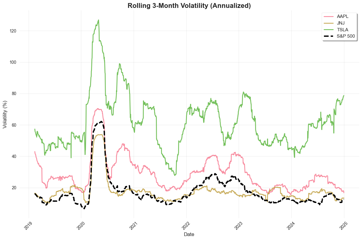
Plot 7: Matplotlib - Rolling Volatility#
Let’s visualize the rolling volatility using matplotlib.
# Plot 7: Matplotlib - Rolling Volatility
plt.figure(figsize=(12, 8))

for ticker in selected_stocks:
    ticker_data = stock_vol[stock_vol['ticker'] == ticker]
    plt.plot(ticker_data['dlycaldt'], ticker_data['rolling_vol_annual'] * 100,
             label=ticker, linewidth=2, alpha=0.8)

# Add market volatility
plt.plot(market_vol['dlycaldt'], market_vol['rolling_vol_annual'] * 100,
         label='S&P 500', linewidth=3, color='black', linestyle='--')

plt.title('Rolling 3-Month Volatility (Annualized)', fontsize=16, fontweight='bold')
plt.xlabel('Date', fontsize=12)
plt.ylabel('Volatility (%)', fontsize=12)
plt.legend(fontsize=11, frameon=True, fancybox=True, shadow=True)
plt.grid(True, alpha=0.3)
plt.xticks(rotation=45)
plt.tight_layout()
plt.show()
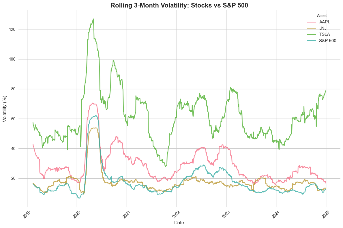
Plot 8: Seaborn - Volatility Comparison#
Now let’s use Seaborn for the volatility visualization.
# Plot 8: Seaborn - Volatility Comparison
plt.figure(figsize=(12, 8))
sns.set_style("whitegrid")

# Prepare volatility data for seaborn
vol_plot_data = []
for ticker in selected_stocks:
    ticker_data = stock_vol[stock_vol['ticker'] == ticker][['dlycaldt', 'rolling_vol_annual']]
    ticker_data['ticker'] = ticker
    vol_plot_data.append(ticker_data)

# Add market volatility
market_vol_data = market_vol[['dlycaldt', 'rolling_vol_annual']].copy()
market_vol_data['ticker'] = 'S&P 500'
vol_plot_data.append(market_vol_data)

vol_plot_df = pd.concat(vol_plot_data, ignore_index=True)
vol_plot_df['rolling_vol_annual'] = vol_plot_df['rolling_vol_annual'] * 100  # Convert to percentage

sns.lineplot(data=vol_plot_df, x='dlycaldt', y='rolling_vol_annual', hue='ticker',
             linewidth=2, alpha=0.8)

plt.title('Rolling 3-Month Volatility: Stocks vs S&P 500', fontsize=16, fontweight='bold')
plt.xlabel('Date', fontsize=12)
plt.ylabel('Volatility (%)', fontsize=12)
plt.legend(title='Asset', fontsize=11)
plt.xticks(rotation=45)
plt.tight_layout()
plt.show()
Plot 9: Plotly Express - Interactive Volatility#
Finally, let’s create an interactive volatility plot with Plotly.
# Plot 9: Plotly Express - Interactive Volatility
fig = px.line(vol_plot_df, x='dlycaldt', y='rolling_vol_annual', color='ticker',
              title='Interactive Rolling Volatility Analysis',
              labels={'dlycaldt': 'Date', 'rolling_vol_annual': 'Volatility (%)', 'ticker': 'Asset'},
              line_shape='linear', render_mode='svg')

fig.update_layout(
    title_font_size=16,
    xaxis_title_font_size=12,
    yaxis_title_font_size=12,
    legend_title_font_size=12,
    hovermode='x unified'
)

fig.show()
Summary Statistics#
Let’s compile a comprehensive summary of our analysis results.
# Summary statistics
print("\n=== Summary Statistics ===")
print("Cumulative Returns (as of latest date):")
for ticker in selected_stocks:
    latest_ret = stock_cumret[stock_cumret['ticker'] == ticker]['cumret'].iloc[-1]
    print(f"{ticker}: {latest_ret:.2f}x")

latest_market_ret = market_cumret['cumret'].iloc[-1]
print(f"S&P 500: {latest_market_ret:.2f}x")

print("\nTotal Dividends Paid:")
for ticker in selected_stocks:
    total_div = stock_cumdiv[stock_cumdiv['ticker'] == ticker]['cumdiv'].iloc[-1]
    print(f"{ticker}: ${total_div:.2f}")

print("\nAverage Annualized Volatility (3-month rolling):")
for ticker in selected_stocks:
    avg_vol = stock_vol[stock_vol['ticker'] == ticker]['rolling_vol_annual'].mean() * 100
    print(f"{ticker}: {avg_vol:.1f}%")

avg_market_vol = market_vol['rolling_vol_annual'].mean() * 100
print(f"S&P 500: {avg_market_vol:.1f}%")
=== Summary Statistics ===
Cumulative Returns (as of latest date):
AAPL: 6.65x
JNJ: 1.32x
TSLA: 18.20x
S&P 500: 2.35x

Total Dividends Paid:
AAPL: $9.37
JNJ: $25.98
TSLA: $0.00

Average Annualized Volatility (3-month rolling):
AAPL: 29.0%
JNJ: 17.7%
TSLA: 61.6%
S&P 500: 17.5%
Analysis Complete#
This script demonstrates:
Matplotlib plotting with pyplot interface
Seaborn plotting with enhanced styling
Plotly Express for interactive visualizations
Cumulative return analysis for selected stocks vs S&P 500
Dividend analysis comparing dividend-paying vs non-dividend stocks
Rolling volatility analysis using 3-month windows
The analysis provides insights into:
Performance comparison between different types of stocks
Income generation through dividends
Risk characteristics over time
Interactive visualization capabilities for data exploration “””
print(“\n=== Analysis Complete ===”) print(“This script demonstrates:”) print(“1. Matplotlib plotting with pyplot interface”) print(“2. Seaborn plotting with enhanced styling”) print(“3. Plotly Express for interactive visualizations”) print(“4. Cumulative return analysis for selected stocks vs S&P 500”) print(“5. Dividend analysis comparing dividend-paying vs non-dividend stocks”) print(“6. Rolling volatility analysis using 3-month windows”)