Data Module Integration Tests

This notebook provides integration tests for the finm.data module by:

1. Pulling each data source

2. Creating simple visualizations

3. Calculating factor exposures for asset return data

Data Sources:

• Factor Data: Fama-French 3 factors, Federal Reserve yield curve, He-Kelly-Manela factors

• Asset Returns: Open Source Bond (treasury and corporate returns)

import os
from pathlib import Path

import matplotlib.pyplot as plt
import pandas as pd
from dotenv import load_dotenv

import finm
from finm.data import fama_french, federal_reserve, he_kelly_manela, open_source_bond

load_dotenv()

DATA_DIR = Path(os.environ.get("DATA_DIR", "./_data"))
DATA_DIR.mkdir(parents=True, exist_ok=True)

print(f"Data directory: {DATA_DIR}")

Data directory: /Users/jbejarano/GitRepositories/finm/_data

1. Fama-French Factors

The Fama-French 3-factor model provides:

• Mkt-RF: Market excess return

• SMB: Small Minus Big (size factor)

• HML: High Minus Low (value factor)

• RF: Risk-free rate

# Load Fama-French data from bundled data (data_dir=None)
ff_factors = fama_french.load(
    data_dir=None,
).to_pandas()
ff_factors = ff_factors.set_index("Date")
print(f"Loaded Fama-French factors (converted to pandas DataFrame)")
print(f"\nFama-French factors shape: {ff_factors.shape}")
print(f"Columns: {ff_factors.columns}")
ff_factors.head()

Loaded Fama-French factors (converted to pandas DataFrame)

Fama-French factors shape: (1227, 4)
Columns: Index(['Mkt-RF', 'SMB', 'HML', 'RF'], dtype='object')

	Mkt-RF	SMB	HML	RF
Date
2021-01-12	0.0037	0.0128	0.0124	0.0
2021-01-13	0.0006	-0.0094	-0.0045	0.0
2021-01-14	-0.0012	0.0202	0.0113	0.0
2021-01-15	-0.0086	-0.0050	-0.0074	0.0
2021-01-19	0.0092	0.0088	-0.0079	0.0

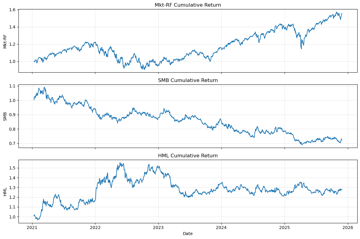
# Plot Fama-French factors
fig, axes = plt.subplots(3, 1, figsize=(12, 8), sharex=True)

# Cumulative returns for each factor
for ax, factor in zip(axes, ["Mkt-RF", "SMB", "HML"]):
    cumulative = (1 + ff_factors[factor]).cumprod()
    ax.plot(cumulative.index, cumulative.values)
    ax.set_ylabel(factor)
    ax.set_title(f"{factor} Cumulative Return")
    ax.grid(True, alpha=0.3)

plt.xlabel("Date")
plt.tight_layout()
plt.show()

# Summary statistics
print("\nFama-French Factor Statistics (Daily):")
print(ff_factors[["Mkt-RF", "SMB", "HML", "RF"]].describe())

Fama-French Factor Statistics (Daily):
            Mkt-RF          SMB          HML           RF
count  1227.000000  1227.000000  1227.000000  1227.000000
mean      0.000424    -0.000233     0.000245     0.000129
std       0.011242     0.007336     0.009452     0.000092
min      -0.059200    -0.027000    -0.038900     0.000000
25%      -0.005150    -0.005200    -0.005500     0.000000
50%       0.000500    -0.000500    -0.000100     0.000200
75%       0.006600     0.004200     0.005800     0.000200
max       0.096500     0.036100     0.037100     0.000200

2. Federal Reserve Yield Curve

The GSW (Gurkaynak, Sack, Wright) yield curve provides:

• Zero-coupon yields for maturities 1-30 years

• Nelson-Siegel-Svensson model parameters

Note: These are yields, not returns.

# Load Federal Reserve yield curve data with auto-pull
yields = federal_reserve.load(
    data_dir=DATA_DIR,
    variant="standard",
    pull_if_not_found=True,
    accept_license=True,
).to_pandas()
yields = yields.set_index("Date")

print(f"Yield curve shape: {yields.shape}")
print(f"Columns: {yields.columns}")
yields.head()

Yield curve shape: (16843, 30)
Columns: Index(['SVENY01', 'SVENY02', 'SVENY03', 'SVENY04', 'SVENY05', 'SVENY06',
       'SVENY07', 'SVENY08', 'SVENY09', 'SVENY10', 'SVENY11', 'SVENY12',
       'SVENY13', 'SVENY14', 'SVENY15', 'SVENY16', 'SVENY17', 'SVENY18',
       'SVENY19', 'SVENY20', 'SVENY21', 'SVENY22', 'SVENY23', 'SVENY24',
       'SVENY25', 'SVENY26', 'SVENY27', 'SVENY28', 'SVENY29', 'SVENY30'],
      dtype='object')

	SVENY01	SVENY02	SVENY03	SVENY04	SVENY05	SVENY06	SVENY07	SVENY08	SVENY09	SVENY10	...	SVENY21	SVENY22	SVENY23	SVENY24	SVENY25	SVENY26	SVENY27	SVENY28	SVENY29	SVENY30
Date
1961-06-14	2.9825	3.3771	3.5530	3.6439	3.6987	3.7351	3.7612	NaN	NaN	NaN	...	NaN	NaN	NaN	NaN	NaN	NaN	NaN	NaN	NaN	NaN
1961-06-15	2.9941	3.4137	3.5981	3.6930	3.7501	3.7882	3.8154	NaN	NaN	NaN	...	NaN	NaN	NaN	NaN	NaN	NaN	NaN	NaN	NaN	NaN
1961-06-16	3.0012	3.4142	3.5994	3.6953	3.7531	3.7917	3.8192	NaN	NaN	NaN	...	NaN	NaN	NaN	NaN	NaN	NaN	NaN	NaN	NaN	NaN
1961-06-19	2.9949	3.4386	3.6252	3.7199	3.7768	3.8147	3.8418	NaN	NaN	NaN	...	NaN	NaN	NaN	NaN	NaN	NaN	NaN	NaN	NaN	NaN
1961-06-20	2.9833	3.4101	3.5986	3.6952	3.7533	3.7921	3.8198	NaN	NaN	NaN	...	NaN	NaN	NaN	NaN	NaN	NaN	NaN	NaN	NaN	NaN

5 rows × 30 columns

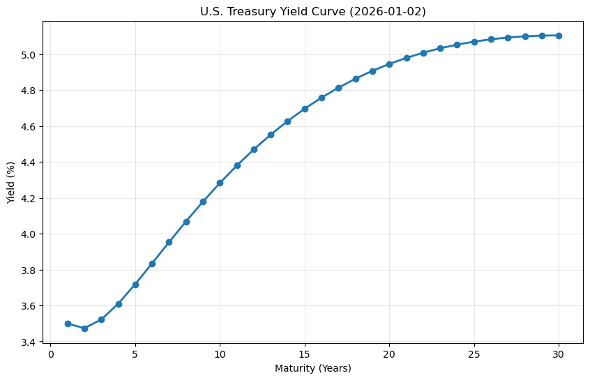
# Plot yield curve snapshot for the most recent date
latest_date = yields.index.max()
latest_yields = yields.loc[latest_date]

maturities = [int(col.replace("SVENY", "")) for col in latest_yields.index]

plt.figure(figsize=(10, 6))
plt.plot(maturities, latest_yields.values, "o-", linewidth=2, markersize=6)
plt.xlabel("Maturity (Years)")
plt.ylabel("Yield (%)")
plt.title(f"U.S. Treasury Yield Curve ({latest_date.strftime('%Y-%m-%d')})")
plt.grid(True, alpha=0.3)
plt.show()

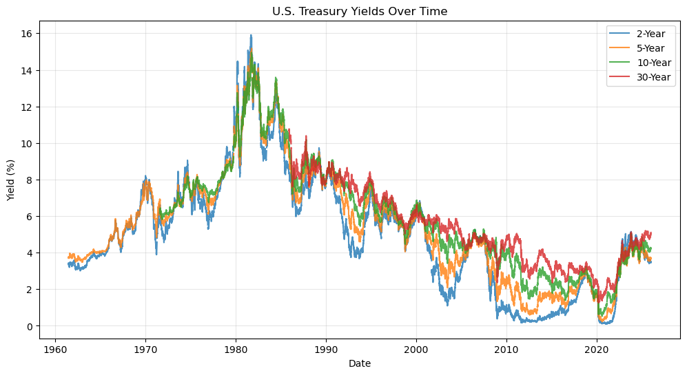
# Plot time series of key maturities
key_maturities = ["SVENY02", "SVENY05", "SVENY10", "SVENY30"]
labels = ["2-Year", "5-Year", "10-Year", "30-Year"]

plt.figure(figsize=(12, 6))
for col, label in zip(key_maturities, labels):
    if col in yields.columns:
        plt.plot(yields.index, yields[col], label=label, alpha=0.8)

plt.xlabel("Date")
plt.ylabel("Yield (%)")
plt.title("U.S. Treasury Yields Over Time")
plt.legend()
plt.grid(True, alpha=0.3)
plt.show()

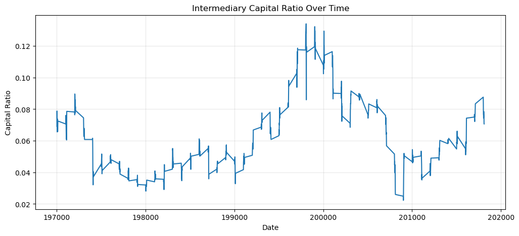
3. He-Kelly-Manela Intermediary Factors

The HKM factors capture:

• Intermediary capital ratio: Capital of financial intermediaries

• Intermediary capital risk factor: Innovation in capital ratio

Note: These are factors, not asset returns.

# Load He-Kelly-Manela data with auto-pull
hkm_monthly = he_kelly_manela.load(
    data_dir=DATA_DIR,
    variant="factors_monthly",
    pull_if_not_found=True,
    accept_license=True,
).to_pandas()
hkm_monthly = hkm_monthly.set_index("yyyymm")

print(f"HKM monthly factors shape: {hkm_monthly.shape}")
print(f"Columns: {hkm_monthly.columns}")
hkm_monthly.head()

HKM monthly factors shape: (587, 5)
Columns: Index(['intermediary_capital_ratio', 'intermediary_capital_risk_factor',
       'intermediary_value_weighted_investment_return',
       'intermediary_leverage_ratio_squared', 'date'],
      dtype='object')

	intermediary_capital_ratio	intermediary_capital_risk_factor	intermediary_value_weighted_investment_return	intermediary_leverage_ratio_squared	date
yyyymm
197001	0.0691	-0.0727	-0.0960	209.1790	1970-01-01
197002	0.0788	0.1416	0.1486	161.1352	1970-02-01
197003	0.0756	-0.0360	-0.0088	174.8429	1970-03-01
197004	0.0688	-0.0870	-0.1050	211.3283	1970-04-01
197005	0.0656	-0.0440	-0.0469	232.2706	1970-05-01

# Plot intermediary capital ratio
if "intermediary_capital_ratio" in hkm_monthly.columns:
    plt.figure(figsize=(12, 5))
    plt.plot(hkm_monthly.index, hkm_monthly["intermediary_capital_ratio"])
    plt.xlabel("Date")
    plt.ylabel("Capital Ratio")
    plt.title("Intermediary Capital Ratio Over Time")
    plt.grid(True, alpha=0.3)
    plt.show()
elif "capital_ratio" in hkm_monthly.columns:
    plt.figure(figsize=(12, 5))
    plt.plot(hkm_monthly.index, hkm_monthly["capital_ratio"])
    plt.xlabel("Date")
    plt.ylabel("Capital Ratio")
    plt.title("Intermediary Capital Ratio Over Time")
    plt.grid(True, alpha=0.3)
    plt.show()
else:
    print("Available columns:", list(hkm_monthly.columns))

4. Open Source Bond Returns

The Open Bond Asset Pricing project provides:

• Treasury bond returns: Government bond returns

• Corporate bond monthly returns: Monthly returns with 108 factor signals

• Corporate bond daily prices: Daily prices from TRACE Stage 1

These are asset returns that can be used for factor analysis.

# Load treasury returns with auto-pull if not found locally
treasury = open_source_bond.load(
    data_dir=DATA_DIR,
    variant="treasury",
    pull_if_not_found=True,
    accept_license=True,
).to_pandas()
print(f"Treasury returns shape: {treasury.shape}")
print(f"Treasury columns: {list(treasury.columns[:10])}...")

Treasury returns shape: (2381340, 5)
Treasury columns: ['DATE', 'CUSIP', 'tr_return', 'tr_ytm_match', 'tau']...

# Load corporate bond returns (monthly with factor signals) with auto-pull
corporate = open_source_bond.load(
    data_dir=DATA_DIR,
    variant="corporate_monthly",
    pull_if_not_found=True,
    accept_license=True,
).to_pandas()
print(f"Corporate returns shape: {corporate.shape}")
print(f"Corporate columns: {list(corporate.columns[:10])}...")
corporate.head()

Corporate returns shape: (1859546, 140)
Corporate columns: ['cusip', 'date', 'issuer_cusip', 'permno', 'permco', 'gvkey', '144a', 'country', 'call', 'ret_vw']...

	cusip	date	issuer_cusip	permno	permco	gvkey	144a	country	call	ret_vw	...	imom1	imom3_1	imom12_1	iltr48_12	iltr30_6	iltr24_3	var_90	es_90	var_95	str
0	000336AE7	2002-08-31	000336	75188.0	NaN	NaN	0	USA	1	0.007252	...	0.009089	0.016714	0.070078	0.259947	0.250910	0.202824	0.032174	0.035203	0.038233	0.051041
1	000336AE7	2002-09-30	000336	75188.0	NaN	NaN	0	USA	1	-0.054660	...	0.015736	0.024968	0.075254	0.263304	0.213676	0.196803	0.038233	0.046446	0.054660	-0.002936
2	000336AE7	2002-10-31	000336	75188.0	NaN	NaN	0	USA	1	0.051999	...	0.014274	0.030234	0.067641	0.295979	0.237394	0.206790	0.038233	0.046446	0.054660	0.066941
3	000336AE7	2002-11-30	000336	75188.0	NaN	NaN	0	USA	1	0.080557	...	0.001263	0.015555	0.075689	0.260612	0.262213	0.207362	0.038233	0.046446	0.054660	0.045280
4	000336AE7	2003-04-30	000336	75188.0	NaN	NaN	0	USA	1	0.067899	...	0.005471	0.018439	0.120662	0.257004	0.244847	0.196972	0.038233	0.046446	0.054660	0.053730

5 rows × 140 columns

# Plot treasury returns if available
if "bond_ret" in treasury.columns:
    # Aggregate treasury returns
    treasury_agg = treasury.groupby("date")["bond_ret"].mean()

    plt.figure(figsize=(12, 5))
    cumulative = (1 + treasury_agg).cumprod()
    plt.plot(cumulative.index, cumulative.values)
    plt.xlabel("Date")
    plt.ylabel("Cumulative Return")
    plt.title("Average Treasury Bond Cumulative Returns")
    plt.grid(True, alpha=0.3)
    plt.show()
elif "ret" in treasury.columns:
    treasury_agg = treasury.groupby("date")["ret"].mean()

    plt.figure(figsize=(12, 5))
    cumulative = (1 + treasury_agg).cumprod()
    plt.plot(cumulative.index, cumulative.values)
    plt.xlabel("Date")
    plt.ylabel("Cumulative Return")
    plt.title("Average Treasury Bond Cumulative Returns")
    plt.grid(True, alpha=0.3)
    plt.show()
else:
    print("Treasury columns:", list(treasury.columns))

Treasury columns: ['DATE', 'CUSIP', 'tr_return', 'tr_ytm_match', 'tau']

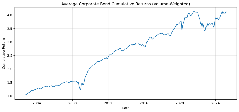
# Plot corporate bond returns
# Note: Monthly corporate data uses ret_vw (volume-weighted total return)
ret_col = "ret_vw" if "ret_vw" in corporate.columns else "bond_ret"
if ret_col in corporate.columns:
    # Aggregate corporate returns by date (equal-weighted across bonds)
    corp_agg = corporate.groupby("date")[ret_col].mean()

    plt.figure(figsize=(12, 5))
    cumulative = (1 + corp_agg.dropna()).cumprod()
    plt.plot(cumulative.index, cumulative.values)
    plt.xlabel("Date")
    plt.ylabel("Cumulative Return")
    plt.title("Average Corporate Bond Cumulative Returns (Volume-Weighted)")
    plt.grid(True, alpha=0.3)
    plt.show()
else:
    print("Corporate columns:", list(corporate.columns))

5. Factor Analysis (Asset Returns Only)

We calculate factor exposures for bond returns against the Fama-French factors. This analysis only applies to asset return data (Open Source Bond), not to yields (Federal Reserve) or factor data (HKM).

# Prepare Fama-French factors for merging
# Resample to monthly if needed for bond data
ff_monthly = ff_factors.resample("ME").last()
print(f"Monthly FF factors shape: {ff_monthly.shape}")

Monthly FF factors shape: (59, 4)

# Calculate factor exposures for corporate bonds
# Note: Monthly corporate data uses ret_vw (volume-weighted total return)
corp_ret_col = "ret_vw" if "ret_vw" in corporate.columns else "bond_ret"
if corp_ret_col in corporate.columns and "date" in corporate.columns:
    # Aggregate corporate returns by date (equal-weighted portfolio)
    corp_monthly = corporate.groupby("date")[corp_ret_col].mean()
    corp_monthly.index = pd.to_datetime(corp_monthly.index)

    # Resample to month-end to align with FF factors
    corp_monthly = corp_monthly.resample("ME").mean()

    # Calculate factor exposures
    exposures_corp = finm.calculate_factor_exposures(
        corp_monthly,
        ff_monthly,
        annualization_factor=12.0,  # Monthly data
    )

    print("\nCorporate Bond Factor Exposures:")
    print("-" * 40)
    for key, value in exposures_corp.items():
        print(f"  {key}: {value:.4f}")

Corporate Bond Factor Exposures:
----------------------------------------
  average_return: 0.0052
  volatility: 0.0755
  sharpe_ratio: 0.0511
  market_beta: 1.0169
  smb_beta: -1.3948
  hml_beta: 0.0425

# Calculate factor exposures for treasury bonds
if "bond_ret" in treasury.columns:
    # Aggregate treasury returns by date
    treas_monthly = treasury.groupby("date")["bond_ret"].mean()
    treas_monthly.index = pd.to_datetime(treas_monthly.index)
    treas_monthly = treas_monthly.resample("ME").mean()

    exposures_treas = finm.calculate_factor_exposures(
        treas_monthly, ff_monthly, annualization_factor=12.0
    )

    print("\nTreasury Bond Factor Exposures:")
    print("-" * 40)
    for key, value in exposures_treas.items():
        print(f"  {key}: {value:.4f}")
elif "ret" in treasury.columns:
    treas_monthly = treasury.groupby("date")["ret"].mean()
    treas_monthly.index = pd.to_datetime(treas_monthly.index)
    treas_monthly = treas_monthly.resample("ME").mean()

    exposures_treas = finm.calculate_factor_exposures(
        treas_monthly, ff_monthly, annualization_factor=12.0
    )

    print("\nTreasury Bond Factor Exposures:")
    print("-" * 40)
    for key, value in exposures_treas.items():
        print(f"  {key}: {value:.4f}")

# Summary comparison table
if "exposures_corp" in dir() and "exposures_treas" in dir():
    summary = pd.DataFrame(
        {
            "Corporate Bonds": exposures_corp,
            "Treasury Bonds": exposures_treas,
        }
    ).T

    print("\nFactor Exposure Comparison:")
    print("=" * 60)
    print(summary.to_string())

6. WRDS Data (Optional)

WRDS data requires authentication. This section is skipped if credentials are not available.

# Check for WRDS credentials
WRDS_USERNAME = os.environ.get("WRDS_USERNAME", "")

if WRDS_USERNAME:
    print(f"WRDS username found: {WRDS_USERNAME}")
    print("WRDS data pull is available but skipped in this notebook.")
    print("To pull WRDS data, use:")
    print("  from finm.data import wrds")
    print(
        "  wrds.pull(data_dir=DATA_DIR, variant='treasury', wrds_username=WRDS_USERNAME)"
    )
else:
    print("WRDS credentials not found.")
    print("To use WRDS data, set the WRDS_USERNAME environment variable:")
    print("  export WRDS_USERNAME=your_username")
    print("Or add to your .env file:")
    print("  WRDS_USERNAME=your_username")

WRDS username found: jmbejara
WRDS data pull is available but skipped in this notebook.
To pull WRDS data, use:
  from finm.data import wrds
  wrds.pull(data_dir=DATA_DIR, variant='treasury', wrds_username=WRDS_USERNAME)

Summary

This notebook demonstrated:

1. Fama-French Factors: Loaded and visualized the 3-factor model data

2. Federal Reserve Yield Curve: Downloaded GSW yields and plotted the term structure

3. He-Kelly-Manela Factors: Pulled intermediary capital factor data

4. Open Source Bond Returns: Downloaded treasury and corporate bond returns

5. Factor Analysis: Calculated factor exposures for bond returns

All data sources follow the standardized interface:

• pull(data_dir, accept_license=True): Download data from source

• load(data_dir, variant, pull_if_not_found, accept_license): Load cached data (returns polars DataFrame)

• to_long_format(df): Convert to long format

Note: When using pull_if_not_found=True, you must also set accept_license=True to acknowledge the data provider’s licensing terms. See each module’s LICENSE_INFO for details.